ZHANG Xiao-xi (張曉曦), CHENG Yong-guang (程永光), YANG Jian-dong (楊建東),

XIA Lin-sheng (夏林生), LAI Xu (賴旭)

State Key Laboratory of Water Resources and Hydropower Engineering Science, Wuhan University, Wuhan 430072, China, E-mail: zhangxiaoxi@whu.edu.cn

Simulation of the load rejection transient process of a francis turbine by using a 1-D-3-D coupling approach*

ZHANG Xiao-xi (張曉曦), CHENG Yong-guang (程永光), YANG Jian-dong (楊建東),

XIA Lin-sheng (夏林生), LAI Xu (賴旭)

State Key Laboratory of Water Resources and Hydropower Engineering Science, Wuhan University, Wuhan 430072, China, E-mail: zhangxiaoxi@whu.edu.cn

(Received February 22, 2013, Revised March 24, 2013)

This paper presents the simulation and the analysis of the transient process of a Francis turbine during the load rejection by employing a one-dimensional and three-dimensional (1-D-3-D) coupling approach. The coupling is realized by partly overlapping the 1-D and 3-D parts, the water hammer wave is modeled by defining the pressure dependent density, and the guide vane closure is treated by a dynamic mesh method. To verify the results of the coupling approach, the transient parameters for both typical models and a real power station are compared with the data obtained by the 1-D approach, and good agreements are found. To investigate the differences between the transient and steady states at the corresponding operating parameters, the flow characteristics inside a turbine of the real power station are simulated by both transient and steady methods, and the results are analyzed in details. Our analysis suggests that there are just a little differences in the turbine outer characteristics, thus the traditional 1-D method is in general acceptable. However, the flow patterns in the spiral casing, the draft tube, and the runner passages are quite different: the transient situation has obvious water hammer waves, the water inertia, and some other effects. These may be crucial for the draft tube pulsation and need further studies.

Francis turbine, hydraulic transients, CFD simulation, flow characteristics

Introduction

Transient processes are always among the top priorities during the design phases of hydraulic turbines and hydropower stations because they may cause serious accidents[1,2]. Traditionally, the transients in hydropower systems were simulated by 1-D method of characteristics (MOC)[2], in which the transient turbine boundary conditions were represented by steady performance characteristics. This static 1-D description is inadequate to represent the dynamic 3-D characteristics of a turbine when analyzing some special transient phenomena such as the draft tube vortex, the cavitation, the pressure pulsation, and the unit vibration. In these cases, 3-D CFD simulations should be used.

Four key issues must be addressed before using the CFD to simulate turbine transients: how to define the varying rotational speed of the turbine unit, how to realize the movements of guide vanes, how to consider the dynamic responses of the long pipes from a local turbine, and how to model the acoustic wave of the water hammer. The first two issues can be conveniently addressed by user-defined functions (UDF) in some existing software, such as FLUENT and CFX. These methods were successfully used to simulate the turbine transient processes of the unit start up[3], the runaway[4-6], and the load rejection[7,8]. The third issue is extremely important for simulating the turbine transients in long water conveying systems. However, it is neither necessary nor feasible to model the whole system using the 3-D method. As a solution to this issue, Ruprecht and Helmrich[9]proposed a method to couple the 1-D MOC with the 3-D CFD model when studying the pressure fluctuations in a draft tube. Panov et al.[10]used this method to simulate the draft tube vortex ropes under part-load operating states. Thismethod is relatively simple to formulate and implement. However, the discharge on the 1-D-3-D coupling boundary is computed by assuming that the pressure at the current time step is equal to that of the previous time step. This assumption is not accurate in the physical sense, and therefore not reliable. Yuan et al.[11]provided a coupling method by iteration in the software FLUENT and used it for the simulation of the surge tank oscillations. Fan et al.[12]used the same method to simulate the turbine transient process of the load rejection. Wu et al.[13]developed another iteration method and coupled the 1-D software FLOWMASTER and FLUENT for simulating the transients of a pump system. These two iteration methods have a more rigorous theoretical basis. But they are also more complex and the convergence and the accuracy of the methods are not discussed. Recently Zhang et al.[14]presented two explicit 1-D-3-D coupling methods and their efficiency and accuracy were verified by simulating surge tank transient flows. But the methods have not been used in simulating the turbine transients. The fourth problem, related to introducing the water compressibility into the 3-D CFD model, is the essence of any 3-D simulation of hydraulic transients. Yan et al.[15]and Yin et al.[16]solved the water state equation in CFX and FLUENT. Both of them simulated the pressure fluctuations of the pump-turbine in steady operating states. However, there are few reports of using this treatment for 3-D transient simulations. Therefore, developing an accurate and efficient 1-D-3-D coupling method with a reliable compressible water model is still a challenge in simulating the 3-D transients of turbines.

In this study, the transient process of a Francis turbine during the load rejection is simulated by adopting the optimal 1-D-3-D coupling method with the compressible water model for the first time. The equivalence of the new approach and the conventional 1-D MOC is discussed, and the flow characteristics are compared within the turbine between transient and steady operating states with the same operating parameters.

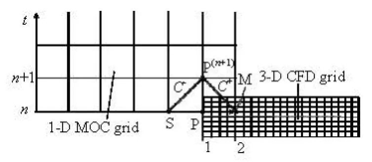
Fig.1 Schematic diagram of the partly overlapped 1-D and 3-D coupling

1. Methods

1.11-D-3-D coupling method

The key problem for the 1-D-3-D coupling is to solve the flow variables on the interfacial boundary. At present, there are several methods as mentioned in the Introduction, among which the partly overlapped coupling (POC) method[14]is physically reliable and straightforward in programming because it solves the discharge and the pressure on the coupling boundary explicitly. Because of its superior accuracy and efficiency, this method is adopted here in our study.

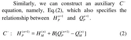
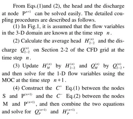
Assume a simple system consisting of a 1-D MOC domain upstream and a 3-D CFD domain downstream (see Fig.1) where the 3-D grid and 1-D grid are overlapped within a single 1-D grid length. We use a section of CFD grid (Section 1-2) to model a MOC grid (Section PM) in order to obtain the discharge and the pressure on the boundaries of the two parts simultaneously. At time step n, the flow variables are known at all grid nodes, including the 1-D and 3-D parts. Therefore, for the 1-D part, the C+equation, namely Eq.(1), can be constructed between nodes S and P(n+1), which gives a relationship between the discharge QP(n+1)and the piezometric head HP(n+1)at time step n+1.

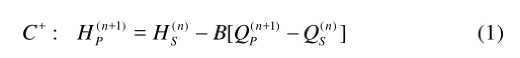
where B=a/(gA), a is the acoustic wave speed, g is the gravity, and A is the area. The superscript is the time step and the subscript is the section index. The head loss is ignored here because the distance between the two nodes is very short.

1.2Compressible water model

The water compressibility and the pipe elasticity are related to the wave speed of the water hammer. To model the 3-D water hammer, the relationship between the density and the pressure, namely, the state equation, should be properly added to the continuity and momentum equations for a CFD simulation. Zhang et al.[19]proposed two methods for modeling the compressible water within software FLUENT. The one by defining density function (DDF) has a clear physical meaning and is proved to be stable and accurate. It is briefly described here.

The state equation for the water is given as[2]

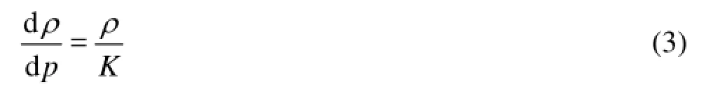
where ρ is the density, p is the relative pressure, and K is the bulk modulus of elasticity. Solving Eq.(3), we obtain

where p0and ρ0are the relative pressure and the density in the initial state, respectively. In addition, underothe standard condition of an ambient temperature 20C and an absolute atmospheric pressure, the value of p0is 0 Pa and ρ0is 998.2 kg/m3.

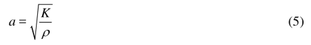
For the water, the change in a is so small that it could be regarded as a known constant, therefore, Eq.(5) can be rewritten as

where a0is the acoustic wave speed in the initial state. Substituting Eq.(6) into Eq.(4), we obtain

For the water enclosed in a finite domain, the wall elasticity may be taken into account by calculating the wave speed0a based on the equation in Ref.[2].

The software FLUENT provides a user-defined density function, which enables the user to customize the density as a function of other flow variables. Here we take Eq.(7) as the density function and solve it explicitly after the pressure p is obtained at every step.

2. Verifications

Here we use several benchmark examples to verify the accuracy of the above proposed models.

2.1Verification of the DDF method

The simple single pipe water hammer phenomena are simulated by using the 3-D defining density function (DDF) method and the results are verified by the 1-D MOC. Consider a single pipe connecting a reservoir at the upstream end and a valve at the downstream end. The2length is 500 m and the cross-sectional area is 4 m. Two types of water hammer waves, induced by valve closing and opening, respectively, are simulated with wave speed a=1000 m/s . In Case 1, the reservoir water3level is 100 m, the initial maximal discharge is 16 m/s, and the valve opening changes linearly from 1.0 s to 0 s in 5.0 s. In Case 2, the reservoir w3ater level is 400 m, the maximal discharge is 10 m/s, and the valve opening changes linearly from 0.1 s to 1.0 s in 5.0 s. The results are illustrated in Fig.2. It is clear that the pressure head (HCase1and HCase2) histories at the valve are well predicted by the 3-D DDF method. The deviations in the data obtained by the 3-D DDF and the data obtained by the 1-D MOC are very small, with the maximal pressure difference less than 0.2% and 0.3% for Case 1 and Case 2, respectively. Therefore, the 3-D DDF method is reliable and can be used in solving more complex problems.

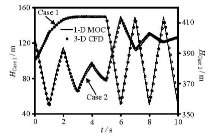
Fig.2 Comparisons of the pressure head at the valve obtained by 3-D DDF and 1-D MOC

2.2Verification of the 1-D-3-D POC method

In Section 2.1, the examples are simulated bydiscretizing the total pipe with the 3-D DDF. In this section the 1-D-3-D partly overlapped coupling (POC) method is used to simulate the same problems. The pipe is bisected, and the two parts are coupled by the 1-D-3-D POC. Figure 3 compares the 1-D-3-D POC results with those obtained by the 1-D MOC, and a good agreement is seen. The data deviations between those obtained by the 1-D-3-D POC and the 1-D MOC are very small, with the maximal pressure difference less than 0.3% and 0.4% for Case 1 and Case 2, respectively. This indicates that the 1-D-3-D POC is reliable in simulating the water hammer phenomena.

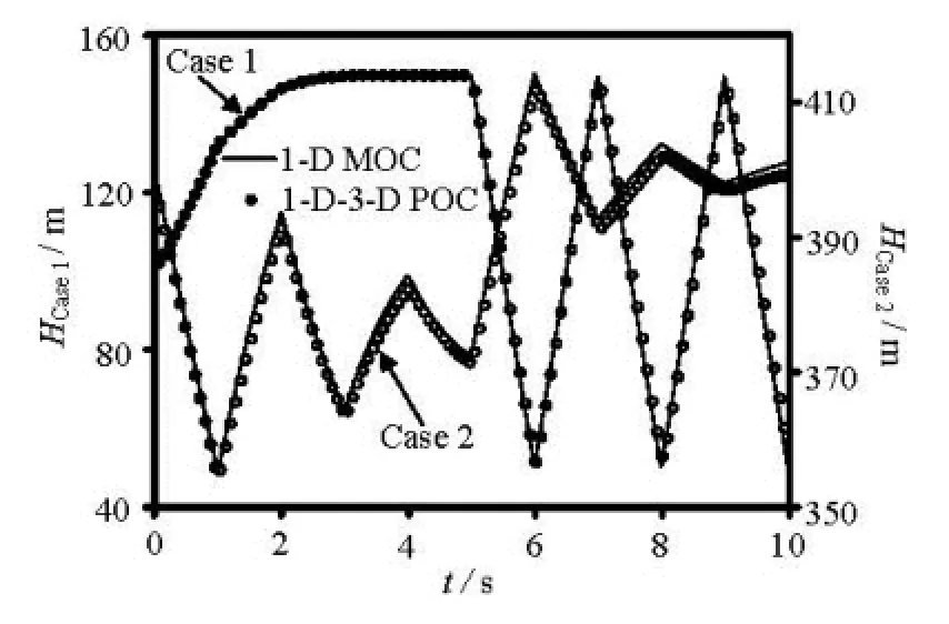
Fig.3 Comparisons of the pressure head at the valve obtained by 1-D MOC and 1-D-3-D POC

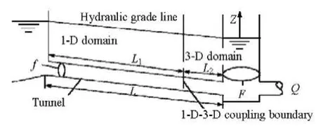
Fig.4 Schematic layout of a simple surge tank

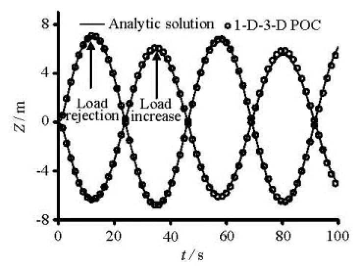
Fig.5 Comparisons of the water level oscillations in the surge tank

To test the ability of the 1-D-3-D POC for simulating the surge tank waves, a simple surge tank oscillation problem is simulated. As shown in Fig.4, the total length of the tunnel (L) is 500 m, including the 1-D part (L1=450 m) and the 3-D part (L2=50 m).

The sectional areas of the tunnel (f) and the surge tank (F) are equal. Under the load rejection condition, the penstock discharge changes linearly from 1.0 m3/s to 0 m3/s in 2.0 s, under the load increase condition, the discharge changes from 0.1 m3/s to 1.0 m3/s in 2.0 s. Figure 5 compares the amplitudes ()Z of the water level oscillations obtained by the 1-D-3-D POC method and the analytic solution of the surge tank equation[2]. The deviations from the analytic solution in the load increase case are 0.17m in the maximal water level and 0.01 m in the minimal water level. In the load rejection case, the deviations in both the maximal and minimal levels are 0.05 m. It is found that the accuracy of the 1-D-3-D POC method is lost a little bit when the ratio of the 3-D part to the whole system becomes larger. However, this ratio in our applications of the 1-D-3-D POC method is always small. Therefore, we may conclude that the 1-D-3-D POC method is capable of simulating the transient problems in hydropower systems.

3. Simulation of the load rejection process of a Francis turbine

3.1Computational conditions

The layout of the hydropower system considered here includes one penstock, one turbine, and one tailrace tunnel,as shown in Fig.6. The turbine, as shown in Fig.7, is simulated by the 3-D CFD software FLUENT, while the penstocks 1, 2, and the tailrace tunnel 2 are simplified to 1-D pipelines and solved by the MOC programmed in UDF of FLUENT. To obtain a uniformly distributed flow on the 1-D-3-D coupling boundaries, the penstock 3 in front of the spiral casing and the tailrace tunnel 1 behind the draft tube, are also treated by the 3-D model. The 1-D-3-D POC method is used to exchange data between the 1-D and 3-D domains. Meanwhile, the DDF method is used to model the water compressibility of the 3-D part and the wave speeds in both domains are defined as 1 000 m/s. The runner rotation and the guide vane’s movements are realized by the dynamic mesh method. The RNG k-ε modelis selected to model the turbulent flow.

In order to select a proper computational grid for the turbine, the grid sensitivity is investigated first by three sets of meshes, and a mesh of 3.4×106cells is finally chosen. The predicted turbine efficiencies (η) on different unit rotational speeds (n1＇) at the opening of 0.275 m are plotted in Fig.8, which shows good agreement between the simulated data and those transformed from the model test results. The relative deviations are below 1.0%.

The initial operating conditions are as follows: the reservoir water level is 400 m, the tailrace waterlevel is 205.6 m, and the rotational speed of the unit is 150 r/min. During the load rejection process, the guide vanes close linearly within 12 s, and the rotational speed is defined by the equation of the rotational acceleration[2]. In the entire simulation process, the time step is fixed to 2×10-4s, which is proper according to our previous studies.

Fig.6 Schematic layout of the whole computational domain

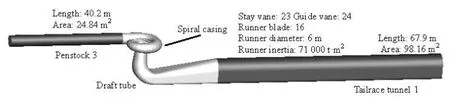
Fig.7 Schematic layout of the 3-D computational domain

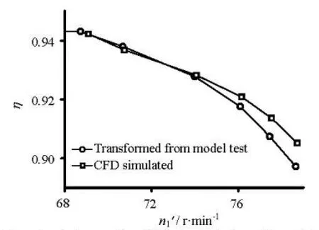
Fig.8 Comparison of the efficiencies between the CFD simulated results and the data transformed from model test

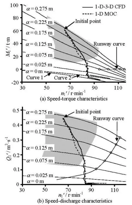
Fig.9 Comparisons of the operating trajectories simulated by 1-D-3-D CFD and 1-D MOC

3.2Results and analyses

3.2.1 Comparisons with the 1-D MOC results

The results obtained by the 1-D MOC are used to verify the 1-D-3-D coupling method. For convenience of comparisons, the initial working head, the discharge, the rotational speed, and the closing rule of the guide vane are kept the same for the two approaches.

The load rejection phenomenon is described as follows. First, the turbine rejects the load suddenly and the guide vanes begin to close. Then, the water hammer waves occur and propagate along the whole hydraulic system; the unit accelerates first and then decelerates gradually after the guide vane’s close. Figure 9 shows the turbine characteristics and the simulated operating trajectories, which are expressed in the unit parameters. The unit torque 1()M＇ and the unit discharge1()Q＇ characteristics of the turbine are shown in Fig.9(a) and Fig.9(b), respectively. The thin curves in the shadow zone are transformed directlyfrom the model turbine hill-chart provided by the turbine manufacturer and the curves outside the shadow zone are extended and interpolated based on the runaway curve and the experience. These characteristics are the basic data to describe the turbine when conducting the 1-D MOC simulation. The trajectory curves in Fig.9 are the simulated results, in which the bold curves are from data obtained by the 1-D-3-D coupling and the dashed curves are from data obtained by the 1-D MOC. These two sets of curves fit well in general, but there are obvious differences in some locations. In the vicinity of zero openings, the evaluated torque curves from the 1-D and 1-D-3-D methods are misaligned, as shown in Fig.9(a). Curve 1 is the zero torque curve extrapolated from larger opening curves, while Curve 2 is the zero opening curve estimated by the 1-D-3-D simulation.

The discharges ()Q obtained by the two methods are depicted in Fig.10(a), and a good agreement between the two curves can be observed. This indicates that the dynamic mesh method can simulate the movements of the guide vanes properly. However, there are some discrepancies in local regions, especially in the small guide vane opening region. This behavior may be attributed to the errors of the extrapolated small opening curves used in the 1-D MOC, and to the errors of the 1-D-3-D CFD in small guide vane openings.

Figure 10(b) shows the histories of the rotational speed ()n obtained by the two methods. The 1-D-3-D data agree well with the 1-D data during the first period of 5 s, and then the two curves begin to diverge. This deviation may be attributed to the different torques by the two methods in the small opening region. The 3-D simulated curve reaches its maximal value 219.7 r/min at 9.7 s and the 1-D curve achieves its maximal value 223.6 r/min at 10.2 s.

Figure 10(c) compares the averaged pressure heads (Hc) at the entrance of the spiral casing. Both curves assume similar shapes during the period of the guide vane closing, and they fit well in the first 4.0 s. During the period of 4.0 s to 6.0 s, the head obtained by 1-D MOC is larger than that by 1-D-3-D CFD. This may be attributed to the larger gradient of the discharge curve of 1-D MOC in Fig.10(a), for the deceleration of the discharge is proportional to the pressure rise of the water hammer. The maximal head obtained by the 1-D-3-D CFD is 264.6 m at about 8.7 s, while that obtained by the 1-D MOC is 268.9 m at about 5.6 s. The difference of 4.3 m is about 2.1% of the working head. After the guide vane is closed at 12 s, the amplitudes of the head fluctuation obtained by the 1-D-3-D CFD are smaller than those obtained by the 1-D MOC. This behavior is due to the different wave reflecting coefficients of the guide vane openings. The cycle of the water hammer wave evaluated by the curves obtained by the 1-D-3-D CFD is 2.4 s. This value matches well with the theoretical value of 2.3 s, which corresponds to the total headrace pipe length of 563.8 m.

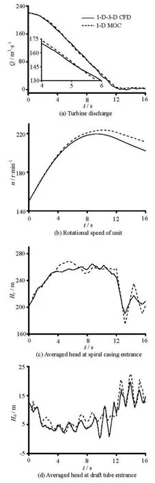
Fig.10 Comparisons of the detailed turbine information obtained by 1-D-3-D CFD and 1-D MOC

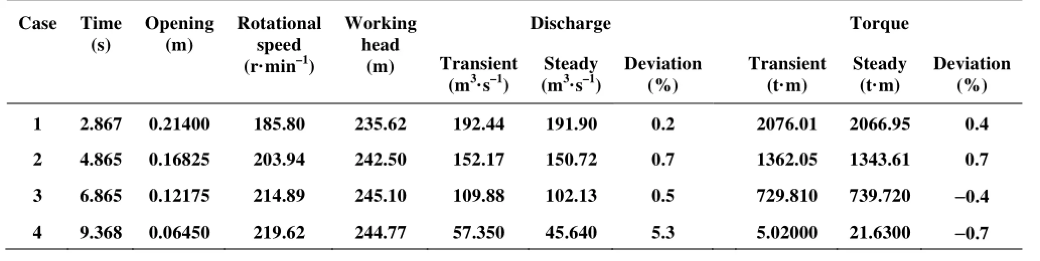
Table1 Comparisons of the turbine performances between transient and steady operating states

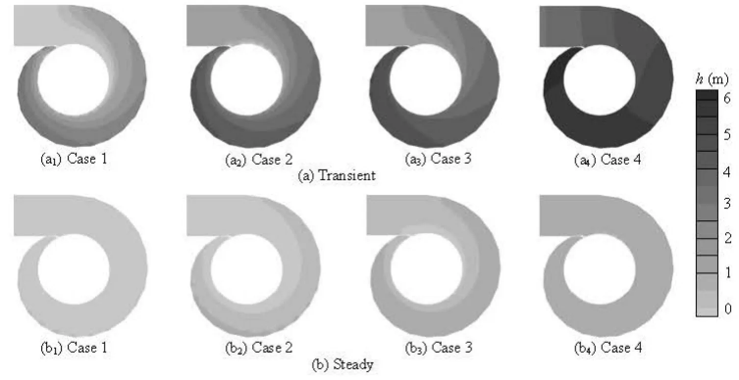
Fig.11 Comparisons of the pressure head distributions in the middle plane of the spiral casing between transient and steady operating states

The head fluctuations at the entrance of the draft tube (Hd) are shown in Fig.10(d). The wave cycles of the two curves all well match the theoretical value of 1.4 s (corresponding to the total tailrace pipe length of 353.1 m), but the head obtained by the 1-D-3-D CFD is lower. The minimal pressure head obtained by the 1-D-3-D CFD is 0.3 m at 9.8 s, which is much lower than 1.9 m at 5.0 s, the one obtained by the 1-D MOC. The smaller pressure head in the draft tube is crucial because it may cause the water column separation, which is related to serious accidents. Because of this, the 1-D-3-D coupling should be applied to investigate the draft tube pressure during the transient process, especially when the pressure value is critical.

Note that the performance of the 1-D MOC simulations shows some uncertainties, especially in the small guide vane opening region, because the characteristics are transformed from the model test data by interpolation, extrapolation, efficiency rectification, and empirical estimation. Therefore, the above general agreements between the results obtained by the 1-D-3-D and the 1-D are sufficient to verify the proposed 1-D-3-D method. Further verification may be conducted in the future.

3.2.2 Comparisons of characteristics between transient and steady states

At present, the transient characteristics of the turbine are estimated and represented by their steady counterparts, which are obtained from small-scale model tests in steady operations. In the above 1-D simulation, the steady characteristic curves in Fig.9 are used as the input data. However, to what extent this representation works well is an important question to be answered. Here, we might discuss the differences of the transient and steady characteristics. Four transient instants in the load rejection process are selected to compare with their corresponding steady operating conditions, in which the working parameters are identical to those in the transient cases. The guide vane openings, the rotational speeds, and the working water heads are listed in Table 1.

There are deviations in the discharges and the torques between the transient and steady operating states, but the deviations are quite small compared to the initial data. Therefore, from the viewpoint of engineering applications, it is well-grounded to conclude thatthere is no obvious difference in the outer characteristics of this turbine between the transient and steady operating states.

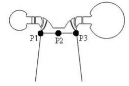
Fig.12 The locations of sensors in the draft tube inlet

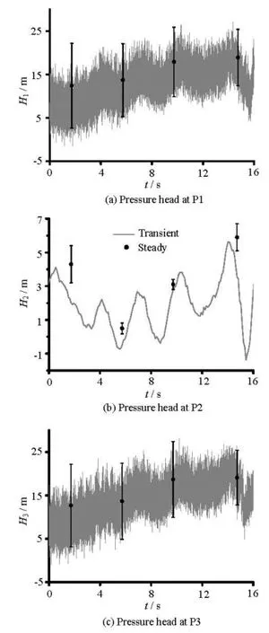
Fig.13 Comparisons of simulated pressure fluctuations at sensor points between transient and steady operating states

During the guide vane closing process, a positive pressure wave propagates from the nose to the entrance of the spiral casing, which leads to the gradual increase of the pressure from the nose to the entrance. Figure 11 shows this phenomenon clearly. In the transient operating state, the pressure in the middle plane of the spiral casing is not uniform, and the increase of the pressure head from the nose to the entrance can be up to 3 m (see Case 4). But in the steady operating state, the pressure is distributed nearly uniformly along the spiral casing centre line. Therefore, the pressure distributions in the turbine are different in the transient and the steady states with the same working parameters. The non-uniform distributions in the transient state are the evidence of the existence of the water hammer effect.

During the guide vane closing process, a negative pressure wave propagates in the draft tube, so the minimal pressure in the draft tube in the transient state is smaller than that in the steady state. Apart from the water hammer effect, there exists the water inertia effect, which is produced by the acceleration of the turbine in the transient state. This effect also influences the pressure distributions in the draft tube. To illustrate this, detailed comparisons are conducted. Three pressure sensors are set in the draft tube entrance: P1 and P3 are at the side and P2 is at the center (see Fig.12). Figure 13 shows the pressure fluctuations (H1, H2and H3) at the sensor points. The black lines are the histories of the pressure head simulated for the transient operating state and the red segments are the fluctuating amplitudes of the pressure head simulated for several selected steady operating cases, in which the operating parameters are the same as those of the corresponding transient instants. It is clear that the pressure variation in the transient and steady states are in general the same, but the mean pressure in the transient sate is lower than that in the steady state. Figure 14 compares the pressure distributions at the draft tube entrance. It is noticed that the pressure distributions in the transient and steady states are entirely different, and the minimal pressure of the transient state is lower than that in the steady state. This discrepancy increases as the guide vane closes. In Case 4, the minimal pressure head in the transient state is about -2 m while that in the steady state is approximately 6 m. Figure 15 depicts these vortex rope shapes defined as the pressure iso-surfaces of 0 Pa in Case 2. Obviously, the vortex rope in the steady state is smaller than that in the transient operating state. Therefore, there are differences in the pressure distributions in the draft tube between the transient and steady states, which is caused not only by the water hammer waves but also by the water inertia.

Generally speaking, the flow patterns in every runner passage are nearly the same according to the rotationally periodic feature of the runner geometry. This is the reason why some CFD simulations wereconducted using a single runner passage. However, we find this rule is not valid in the transient operating regime. Figure 16 depicts the velocity distributions in the middle plane of the runner in the transient and steady operating states. In Cases 1, 2 and 3, the velocity distributions in every runner passage show good periodic features, both in the transient and steady states. But in Case 4, the periodic flow patterns are lost in the transient state, but are kept well in the steady state. This behavior may be attributed to the water inertia and the centrifugal force since the runner speeds up to their maximum rotational speed around the time of this case.

The different number and intensity of the draft tube vortices and the absence of periodicity of the runner flow patterns are important issues that need further studies because they may affect the stability and safety of the turbine.

Through the above comparisons, we may conclude that there is no significant difference in the turbine outer characteristics (such as the torque and the discharge) between the transient and steady operating states with the same operating parameters. However, the flow patterns in the spiral casing, the runner passages, and the draft tube are quite different because of the water hammer wave, the water inertia, and some other factors. Further studies of the transient flow patterns and their effects on the transient process of hydropower systems are necessary.

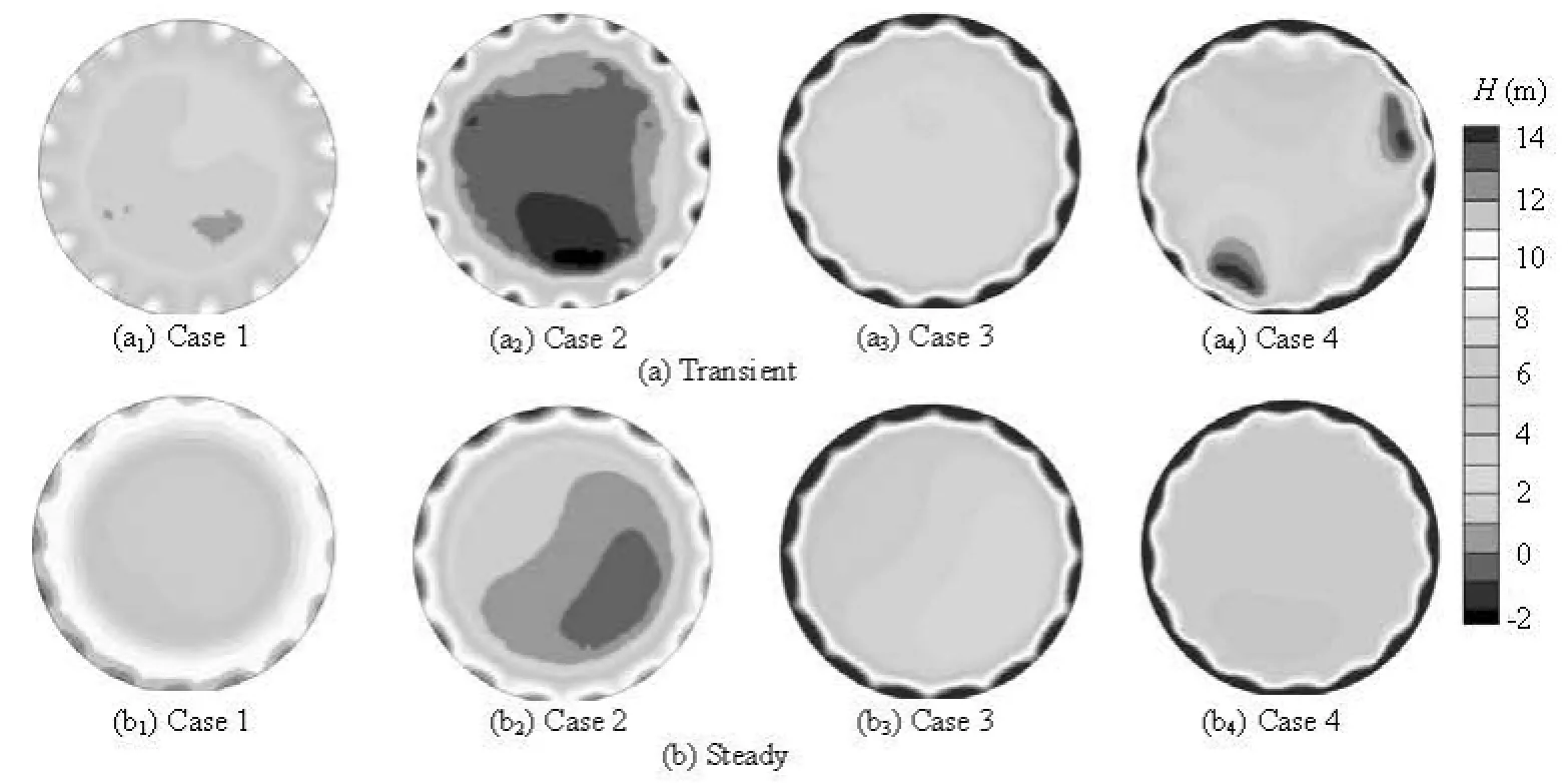
Fig.14 Comparisons of pressure distributions at the draft tube inlet between transient and steady operating states

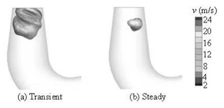
Fig.15 Comparisons of the pressure iso-surface of 0 Pa in draft tube between transient and steady operating states in Case 2

4. Conclusions

In this study, the transient load rejection process of a turbine is simulated by a 1-D-3-D coupling approach and the results of the transient characteristics are compared with those obtained by the traditional 1-D approach and those in the steady states with the same operating parameters.

The results obtained by the 1-D-3-D CFD and 1-D MOC methods agree well qualitatively indicating that the proposed 1-D-3-D coupling method is feasible, reliable, and can be used in engineering applications. Although there is no significant difference in the outer characteristics of the turbine between the transient state and the corresponding steady states, the inner flow patterns inside the turbine are quite different. The special flow patterns in the spiral casing, the runner and the draft tube may be related to the water hammer wave, the water inertia, the centrifugal force, and other effects. The absence of periodicity of the runner flow and the more serious draft tube pressure may be crucial for the stability and safety of hydropower systems. The causes and aftermaths of these special flow patterns, the further validation of the proposed method by mesh refinement studies, the introduction of advanced turbulence models, and the acquisition of more experimental data for comparisons are important studies to be carried out in the future.

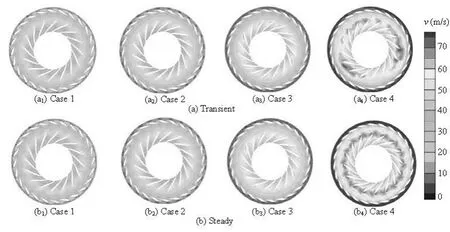
Fig.16 Comparisons of the velocity magnitude contours in the middle plane of the runner between transient and steady operating states

[1] YANG Jian-dong, ZHAO Kun and LI Lin et al. Analysis on the causes of units 7 and 9 accidents at Sayano-Shushenskaya hydropower station[J]. Journal of Hydroelectric Engineering, 2011, 30(4): 226-234(in Chinese).

[2] POPESCU M., ARSENIE D. and VLASE P. Applied hydraulic transients for hydropower plants and pumping stations[M]. Rotterdam, The Netherlands: A. A. Balkema, 2003.

[3] NICOLLE J., MORISSETTE J. F. and GIROUX A. M. Transient CFD simulation of a Francis turbine startup[C]. 26th IAHR Symposium on Hydraulic Machinery and Systems. Beijing, China, 2012.

[4] LIU J., LIU S. and SUN Y. et al. Three-dimensional flow simulation of transient power interruption process of a prototype pump-turbine at pump mode[J]. Journal of Mechanical Science and Technology, 2013, 27(5): 1305-1312.

[5] LI Jin-wei, LIU Shu-hong and ZHOU Da-qing et al. Three-dimensional unsteady simulation of the runaway transient of the Francis turbine[J]. Journal of Hydroelectric Engineering, 2009, 28(1): 178-182(in Chinese).

[6] ZHOU Da-qing, WU Yu-lin and LIU Shu-hong. Threedimensional CFD simulation of the runaway transients of a propeller turbine model[J]. Journal of Hydraulic Engineering, 2010, 41(2): 233-238(in Chinese).

[7] KOL?EK T., DUHOVNIK J. and BERGANT A. Simulation of unsteady flow and runner rotation during shutdown of an axial water turbine[J]. Journal of Hydraulic Research, 2006, 44(1): 129-137.

[8] LIU J., LIU S. and SUN Y. et al. Three dimensional flow simulation of load rejection of a prototype pumpturbine[J]. Engineering with Computers, 2013, 29(4): 417-426.

[9] RUPRECHT A., HELMRICH T. Simulation of the water hammer in a hydro power plant caused by draft tube surge[C]. 4th ASME/JSME Joint Fluids Engineering Conference. Honolulu, Hawaii, USA, 2003.

[10] PANOV L. V., CHIRKOV D. V. and CHERNY S. G. et al. Numerical simulation of pulsation processes in hydraulic turbine based on 3D cavitating flow[J]. Thermophysics and Aeromechanics, 2014, 21(1): 31-43.

[11] YUAN Yi-fa, FAN Hong-guang and LI Feng-chao et al. Study on three-dimensional flow in surge tank with consideration of pipeline property[J]. Journal of Hydroelectric Engineering, 2012, 31(1): 168-172(in Chinese).

[12] FAN Hong-gang, HUANG Wei-de and CHENG Naixiang. Transient simulation of turbine jointed with diversion penstock[J]. Journal of Drainage and Irrigation Machinery Engineering, 2012, 30(6): 695-699(in Chinese).

[13] WU D., LIU Q. and WU P. et al. Simulations on dynamic characteristics of pump and pipe system during pumps and valves adjusting process[C]. 26th IAHR Symposium on Hydraulic Machinery and Systems. Beijing, China, 2012.

[14] ZHANG Xiao-xi, CHENG Yong-guang. Simulation of hydraulic transients in hydropower systems using the 1-D-3-D coupling approach[J]. Journal of Hydrodynamics, 2012, 24(4): 595-604.

[15] YAN J., KOUTNIK J. and SEIDEL U. et al. Compressible simulation of rotor-stator interaction in pump-turbines[C]. 25th IAHR Symposium on Hydraulic Machinery and Systems. Timisoara, Romania, 2010.

[16] YIN J., WANG D. and WANG L. et al. Effects of water compressibility on the pressure fluctuation prediction in pump turbine[C]. 26th IAHR Symposium on Hydraulic Machinery and Systems. Beijing, China, 2012.

10.1016/S1001-6058(14)60080-9

* Project supported by the National Natural Science Foundation of China (Grant Nos. 51039005 and 50909076).

Biography: ZHANG Xiao-xi (1986-), Male, Ph. D. Candidate

CHENG Yong-guang,

E-mail: ygcheng@whu.edu.cn