Jiangshan ZHU,Fanyou KONG,Xiao-Ming HU,Yan GUO,Lingkun RAN,and Hengchi LEI

1Institute of Atmospheric Physics,Chinese Academy of Sciences,Beijing 100029,China

2Center for Analysis and Prediction of Storms,University of Oklahoma,Norman,Oklahoma 73072,USA

3State Key Laboratory of Earth Surface Processes and Resource Ecology,Beijing Normal University,Beijing 100875,China

1.Introduction

Ensemble forecasting is well known in numerical weather prediction(NWP)as a valuable technique for producing probabilistic weather forecasts whilst at the same time providing an estimate of uncertainty in the forecasts.However,ensemble forecasts often suffer from under-dispersion,especially at near-surface levels and in precipitation forecasts,indicating that ensembles do not fully represent uncertainties(e.g.,Hou et al.,2001;Mullen and Buizza,2001).One commonly believed reason is that ensemble forecasts neglect the uncertainties caused by land surface condition errors(Sutton et al.,2006).The land surface condition not only affects the lower levels of the atmosphere,but also has an evident influence on mesoscale circulation,deep convection initiation and precipitation(Segal and Arritt,1992;Pielke,2001;Taylor et al.,2007).Research into explicitly representing land surface uncertainties has been performed for forecasts from short-range(Wang et al.,2010)to climatic(MacLeod et al.,2016;Orth et al.,2016)scales.

In short-range forecasting,coupled land–atmosphere models have been commonly used to improve the simulation of land–atmosphere interaction(Smirnova et al.,1997;Chen and Dudhia,2001).The heat and moisture fluxes from the land surface to the atmosphere in land surface models(LSMs)have been found to be sensitive to several factors,such as land-use type(Cheng et al.,2013;Zhang et al.,2007),initial soil moisture(ISM,Trier et al.,2004,2008;Case et al.,2011),land–atmosphere coupling strength(Chen and Zhang,2009;Trier et al.,2010),and sophistication of the LSM(Trier et al.,2008).Improving the accuracy of these factors can substantially improve the simulation of fluxes between land and atmosphere,and improve the forecasting of atmospheric variables.However,a lack of observations and model shortcomings mean that these high impact factors have inevitable errors,which grow nonlinearly through land–atmosphere interaction,and cause notable uncertainties in many key variables in short-range NWP,such as near-surface variables and quantitative precipitation.

Several studies have attempted to represent these uncertainties in short-range ensemble forecasts(SREFs),most of which have focused on perturbing the ISM.Their methods can be mainly divided into two categories.In the first category,the ensemble ISM is obtained through statistical methods.Aligo et al.(2007)constructed a 10-member ensem-ble by sampling 10 specific percentiles from a normal distribution fitted to three soil moisture analyses.Quintanar and Mahmood(2012)constructed a 12-member ensemble forecast by adding or subtracting a uniform perturbation over the whole model domain from the control forecast member.This approach is useful for understanding the sensitivity of the atmosphere to ISM perturbations.However,the perturbations are probably not compatible with most models.The second category applies the breeding method.Wang et al.(2010)proposed a non-cycling surface breeding strategy for generating natural perturbations for initial soil temperature and moisture.The non-cycling mechanism was designed to address climate drift in regional models.It was implemented and verified in the Aire Limit′ee Adaptation Dynamique D′eveloppement Inter National-Limited Area Ensemble Forecasting system and shown to improve the performance of near-surface variable forecasts and precipitation forecasts.Similarly,but without a non-cycling mechanism,Tennant and Beare(2014)perturbed the soil moisture content in the Met Office Global and Regional Ensemble Prediction System by using difference fields generated in the last cycle as perturbations for the current cycle,which improved the skill of the near-surface temperature forecast.These methods can produce well-organized perturbations that are compatible with models.However,in these studies,the factors used to scale the perturbation amplitudes were arbitrarily set to 1.0,without reference to any analysis of soil moisture uncertainty.

China has some of the strongest land–atmosphere coupling effects in the world(Koster et al.,2004),and several studies have shown that ISM has a significant influence on the numerical simulation of high-impact weather events,such as heat waves(Zeng et al.,2014)and heavy rainfall(Chen et al.,2010;Meng et al.,2012).However,these studies were performed with relatively few soil moisture analyses;one of them compared two different soil analyses(Chen et al.,2010),and the others compared a group of ISMs generated by scaling a single soil moisture analysis with different factors(Meng et al.,2012;Zeng et al.,2014).Moreover,few studies have focused on how the ensemble spread and forecast skill of the SREF would be affected by ISM uncertainty in this region.

In the current study we performed an experiment with ensemble forecasts using five different soil moisture analyses.Specifically, five soil moisture analyses from three operational/research centers[the National Centers for Environmental Prediction(NCEP);the European Centre for Mediumrange Weather Forecasts(ECMWF);and the National Aeronautics and Space Administration(NASA)]were used to initiate ensemble forecasts at convection-allowing resolution and at 4-km grid spacing during a two-month period over a northern China domain during summer 2014.Compared with breeding perturbations generated by a single model,analyses produced by state-of-the-art analysis systems from different operational/research centers may present a more reliable estimation of uncertainty(Ebert,2001).Using these analyses,our aim was to investigate the impact of ISM uncertainty on near-surface variables and precipitation forecasts,and the potential of using multiple soil moisture analyses in SREFs.The findings should prove useful for determining the proper ISM perturbation amplitude for future SREF designs by referring to the variance among different soil moisture analyses.In addition,a second ensemble that consisted of mixed microphysics schemes was also performed as a reference,and with which the ISM-perturbed ensemble was compared.Mixing microphysics schemes is commonly used in SREFs,since precipitation is highly sensitive to the chosen microphysics parameterization(MP)scheme,especially at convection-allowing resolution(Duda et al.,2014).Such a comparison can provide additional understanding on the impact of perturbing ISM in a SREF.

2.Data and methods

2.1.Experimental design

An ensemble forecast experiment with perturbed ISM was performed for northern China for each day from 1 July to 31 August 2014.Northern China lies in the northern part of a land-surface-sensitive area of China(Koster et al.,2004),andhasanenormouspopulationandrapideconomicdevelopment.July and August constitute the major rainy season for this region,when the most active land–atmosphere interactions occur.The ensemble had five ensemble members initiated with a different ISM on each day,the aim being to quantify the short-range impact of ISM uncertainty on the SREF,and is referred to as the ISM-perturbed ensemble(ISMPE).Since the MP scheme has a pronounced impact on the simulation of precipitation,and mixed MP schemes are commonly used in SREFs to improve the ensemble spread,another five-member ensemble forecast con figured with mixed MP schemes was performed,which served as a comparison for ISMPE.This experiment is referred to as the MP-perturbed ensemble(MPPE).All forecasts in the two experiments used the Weather Research and Forecasting(WRF)model with the ARW dynamical core,version 3.7,and ran on three nested domains with resolutions of 36 km,12 km and 4 km,and at 50 vertical levels(Fig.1).The 4-km domain had 271×271 grid points,covering the North China.In this study,only the forecasts of the 4-km domain were examined.All forecasts were initiated at 0000 UTC each day,and integrated for 24 h.The two ensembles had the same control member,which used initial and lateral boundary conditions from the NCEP Final(FNL)Operational Global Analysis(1.0°×1.0°).The physics options for the control member were set as:the RRTMG scheme for shortwave and longwave radiation(Iacono et al.,2008);the WRF double-moment 6-class(WDM6,Lim and Hong,2010)scheme for MP;the Kain–Fristch scheme(Kain,2004)for cumulus cloud(for the 36-km and 12-km grids only);the uni fied Noah LSM for the land surface(Tewari et al.,2004);and the Yonsei University scheme(Hong et al.,2006)for the planetary boundary layer.The WDM6 scheme was chosen because of its good performance in precipitation forecasts in the northern China region(Ma et al.,2012).

In ISMPE,the four perturbed members were initiated with four different soil moisture analyses:the ECMWF ERA-Interim dataset(2.0°× 2.0°;Zuo and Zhang,2009;Dee et al.,2011),and three different products from NASA’s Global Land Data Assimilation System(GLDAS)version 1.0;namely,the Noah(0.25°×0.25°),MOSAIC(1.0°×1.0°)and CLM datasets(1.0°×1.0°;Rodell et al.,2004;Zhu and Shi,2014).Water content was assumed to be evenly distributed in each soil layer of the ERA-Interim,MOSAIC and CLM analyses,and aggregated at the layers of the Noah LSM.The horizontal interpolation was performed by the WRF Preprocessing System.The coefficient of variation(standard deviation divided by the mean)of the five analyses at the top level(0–10 cm below ground)showed that most of the soil moisture difference was located in the transition region from plateau to plain(Fig.2a).The 5th,25th,50th,75th and 95th percentiles of the domain-averaged volumetric soil moisture of the five analyses from 1 July to 31 August 2014 are depicted in Fig.2b,showing the different climatologies of the five analyses.Speci fically,the three GLDAS analyses,produced by offline LSMs,were drier than the ERA-Interim and FNL analyses.In particular,the MOSAIC analysis was a much drier outlier.

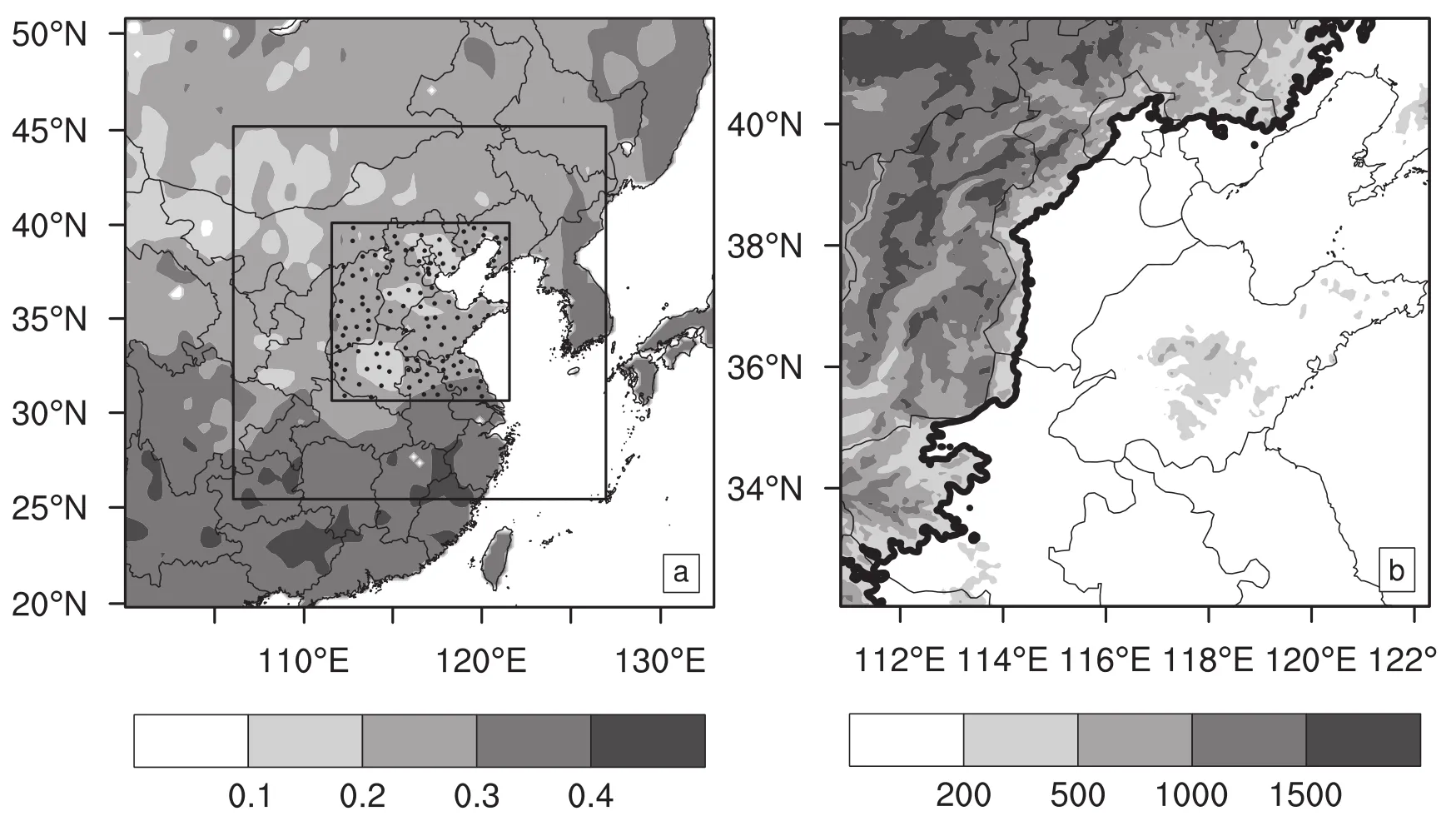
Fig.1.(a)The three nested model domains,land stations(dots),and ISM at 0 to 10 cm below ground for the FNL ensemble member,averaged over all 62 days(shading).(b)Terrain height of the 4-km domain(units:m).The thick line is the 200-m contour line along the Yanshan and Taihang mountains,which divides the domain into the plateau(left)and plain(right).Some small hilly areas were included as part of the plateau for ease of processing(small areas inside the closed contour lines adjacent to the plateau).

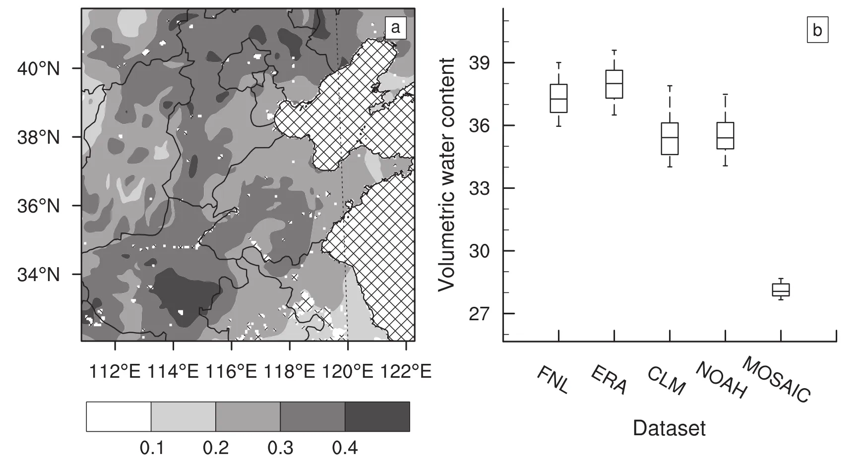
Fig.2.(a)Coefficient of variation of volumetric soil moisture at 0 to 10 cm below ground averaged over 62 days from 1 July 31 August 2014.Water bodies are indicated by the crossed lines.(b)The domain-averaged volumetric soil moisture(%)at 0 to 10 cm below ground of the five analyses over 62 days.The lines indicate the medians,the boxes the 25th and 75th percentiles,and the whiskers the 5th and 95th percentiles.

In MPPE,only the MP scheme was perturbed.The perturbed members used the Thompson(Thompson et al.,2008),Morrison 2-moment(Morrison et al.,2009),Milbrandt–Yau 2-moment(Milbrandt and Yau,2005)and WRF double moment 5-class(Lim and Hong,2010)schemes for the MP option,respectively.

2.2.Veri fication data and method

Observations of temperature and dew point at 2-m above ground(T2mand DPT2m,respectively)and wind speed at 10 m above ground(WIND10m)at 140 stations inside the 4-km domain from 0000 UTC 1 July to 2400 UTC 31 August at 3-h intervals were used to verify the near-surface variables.The locations of the stations are depicted in Fig.1a.The hourly rainfall amount analysis(0.1°×0.1°resolution)issued by the China Meteorological Administration(CMA)was used to verify the precipitation forecast.The analysis was generated by merging hourly rain gauge data at more than 30 000 automatic weather stations in China with the Climate Precipitation Center Morphing precipitation product(Shen et al.,2014;Chen et al.,2016).In this study,the rainfall analysis was interpolated to the 4-km domain before verification.The Gilbert skill score(GSS),also known as the Equitable Threat Score in some literature,and the bias score,were used to examine the skill of the precipitation forecast,while the Brier score(BS)was used to assess the probabilistic precipitation forecast(see Appendix).

3.Results

3.1.Pro files of ensemble spreads

The ensemble spreads(standard deviation across ensemble members)of potential temperature,dew point,U-wind and V-wind,spatially averaged over the land area,were verified for both ISMPE and MPPE at 40 pressure levels from 1000 hPa to 200 hPa,at the forecast times of 6 h and 12 h(1400 LST and 2000 LST,respectively),from 1 July to 31 August 2014.The ensemble spreads for all 62 days were sorted at each level separately,and the 5th percentile,median and 95th percentile are shown in Figs.3 and 4.In general,the ISM perturbation produced a greater ensemble spread at levels below 800 hPa,with the effect decreasing gradually with increasing height.

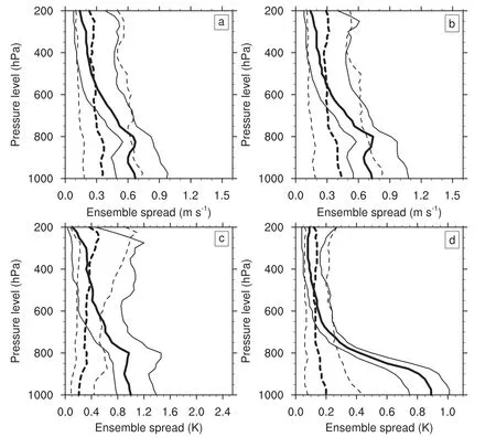
Fig.3.Pro files of the medians(thick line in the middle),5th and 95th percentiles(thin lines on the left and right,respectively)of the ensemble spread of(a)U-wind,(b)V-wind,(c)dew point and(d)potential temperature from ISMPE(solid)and MPPE(dashed)at 6 h,sorted on 62 days from 1 July to 31 August 2014.

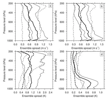
Fig.4.As in Fig.3 but at 18 h.

At 6 h,ISMPE had notable ensemble spread at levels below 800 hPa in all variables.At these levels,the distribution of the ensemble spread was relatively uniform or decreased slowly with height.Above 800 hPa(850 hPa for potential temperature),the ensemble spread decreased more rapidly,indicating that the effects of the ISM perturbation were fading.At 18 h,the ensemble spread increased with time from their values at 6 h at most levels in all the verified variables(Fig.4).However,at the bottom level,the ensemble spread increased less(in wind and dew point)or decreased(in potential temperature),indicating that surface cooling at nighttime constrained the growth of the ensemble spread.

MPPE had a more uniform distribution of ensemble spread at all levels for all variables,except dew point,which had a larger ensemble spread at upper levels.Comparing the two ensembles,the medians of the two ensembles crossed at about 500 hPa.ISMPE had larger ensemble spread below this level,displaying its advantage in producing ensemble spread at the bottom and lower levels of the atmosphere.

3.2.Near-surface variables

The root-mean-square error(RMSE)of the ensemble mean forecasts in ISMPE and MPPE was verified against observations at 140 stations at 3-h intervals from 1 June to 31 August 2014 for T2m,DPT2mand WIND10m(Fig.5).All forecast and observation pairs at the same forecast time on all 62 days were pooled together as verification samples.The ensemble spread was verified for the two ensembles as well.ISMPE had both larger ensemble-mean RMSE and ensemble spread than MPPE in all three verified variables.The differences in ensemble spread were more pronounced than the differences in RMSE between the two ensembles;e.g.,the ensemble spread differences were about twice the magnitude of the ensemble-mean RMSE differences in T2mand DPT2m.On the one hand,the larger ensemble spread in ISMPE indicates soil-moisture perturbation could represent more uncertainty in the near-surface variable forecasts;whilst on the other hand,the larger ensemble-mean RMSE implies more errors were induced in ISMPE.

Fig.5.RMSE of the ensemble mean forecasts(lines)and ensemble spread(marked lines)of ISMPE(solid)and MPPE(dashed)for(a)T2m,(b)DPT2mand(c)WIND10m.

The upward land surface heat and moisture fluxes were averaged over the whole domain and over 62 days for the five members of ISMPE(Fig.6).The three GLDAS members had larger heat fluxes as a result of their drier soil moisture(Fig.2).In particular,the MOSAIC member deviated greatly from the other ensemble members,implying that the MOSAIC analysis is less compatible with Noah LSM.The ensemble members initiated with the ECMWF ERA-Interim,NCEP FNL and GLDAS CLM analyses had comparable performance,with the ERA-Interim member performing the best.The ensemble members that used GLDAS MOSAIC and Noah had obviously larger bias and RMSE in T2mthan other members,and introduced excessive errors into the ensemble,which explains the larger ensemble-mean forecast RMSE in ISMPE.The GLDAS MOSAIC and Noah members performed similarly for DPT2mand WIND10m,and produced larger bias and RMSE than the other members(not shown).It was noted that GLDAS CLM and Noah were similar in their averages(Fig.2),but produced relatively different fluxes and surface temperature biases(Fig.6),implying that the two datasets may have different spatial and temporal patterns.

Previous studies have shown that both bias and stochastic error growth contribute to the ensemble spread,but only stochastic error represents the forecast uncertainty,while the bias only represents forecast error,which should be removed as much as possible(Eckel and Mass,2005).The bias of near-surface variables can be removed reasonably well by subtracting the historical mean bias from the current forecast(Stensrud and Yussouf,2003).In this study,the bias in the ensemble mean RMSE of ISMPE and MPPE was removed by a method similar to that in Stensrud and Yussouf(2003)used for the forecast calibration of near-surface variables.Specifically,the mean bias was calculated for every member of the two ensembles at each grid point and forecast time,by averaging the bias over the 62 days.Then,each mean bias was subtracted from its corresponding forecast.The ensemble-mean forecast RMSE and ensemble spread of the two ensembles were verified again after bias removal(Fig.7).Both the ensemble-mean RMSE and ensemble spread decreased in the two ensembles.The ensemble-mean RMSE of the two ensembles were much closer,indicating that the larger ensemble-mean RMSE of ISMPE was mainly caused by larger biases induced by some of the soil moisture analyses.The ensemble spread differences also decreased but were still notable after bias removal,indicating ISM perturbation carries an advantage in representing stochastic error in nearsurface variable forecasts.

Before and after bias removal,the ensemble spread and ensemble-mean forecast RMSE were closer in ISMPE than MPPE,displaying better statistical consistency in ISMPE.However,ISMPE was still under-dispersed,meaning the uncertainty in near-surface variables was not fully represented by the ISM perturbations.There are several possible explanations for this: first,the five analyses used in this study were not sufficient to fully represent the soil moisture uncertainty;second,other land surface uncertainties were missing, such as uncertainty in land surface characteristics,land–atmosphere coupling strength and the LSM;and third,the lack of perturbation in the atmospheric fields would have constrained the perturbation growth at near-surface levels.

3.3.Precipitation

Figure 8 shows the 24-h accumulated precipitation(APCP24)forecasts of the five members of ISMPE on 14 July 2014,together with the corresponding rainfall analysis.During the day,the edge of the subtropical high was located to the south of the 4-km domain,and a trough at 500 hPa moved from west to east in the domain,caused light to moderate rainfall(about 1 mm to 10 mm)in the north and west of the domain,and moderate to heavy rainfall(about 10 mm to 25 mm)extending southeast of the center of the domain(western Shandong Province),with local maxima exceeding 50 mm.

The five ISMPE members captured the overall precipitation relatively well,though the precipitation was underestimated in the northwest of the domain.The MOSAIC member clearly forecasted less overall precipitation than the other members,implying a drier ISM would probably inhibit summertime precipitation over the domain.Meanwhile,the ensemble members exhibited obvious dispersion in precipitation detail,especially the intensity and location of the local maxima.The FNL,ERA-Interim,and CLM members forecasted similar precipitation in western Shandong Province,which was relatively close to the analysis.The Noah and MOSAIC members had larger southward displacement of the local maxima.The MOSAIC member forecasted the local maxima to lie in Anhui and Jiangsu provinces—much farther south than the other ensemble members and the analysis.

Fig.6.Upward land surface(a)heat flux and(b)moisture flux at the surface,(c)bias,and(d)RMSE of T2mof the five members of ISMPE,temporally averaged from 1 July to 31 August 2014.The fluxes were spatially averaged over land within the 4-km model domain,while the bias and RMSE were averaged over 140 observation stations.

The ensemble spread of the APCP24 forecast was verified for ISMPE and MPPE from 1 July to 31 August 2014 over the 4-km domain,as shown in Fig.9aRainfall analysis was missing for several hours on 15 July 2014 because it is unavailable on the CMA website.along with the domain-averaged daily rainfall amount.ISMPE had comparable ensemble spread to MPPE on most days.ISMPE only had smaller ensemble spread than MPPE for several massive rainfall events when synoptic forcing was relatively strong(e.g.,24July),but still exhibited significant dispersion among the members.

The GSSs and bias scores of the five members of ISMPE were verified for APCP24 exceeding 1 mm,10 mm,25 mm and 50 mm over the 4-km domain.These four thresholds are commonly used in operational forecasting in northern China.All ensemble members except MOSAIC had similar GSSs for all thresholds(Fig.10),indicating these soil moisture analyses produced similar skill in their precipitation forecasts,with none exerting too large a bias.In other words,the probability to be the best forecast was similar among the analyses,which qualified them as ensemble members.The GLDAS MOSAIC member was relatively different from the others,with the lowest GSS for the 1-mm and 10-mm thresholds,but the best GSS for the 50-mm threshold.This is probably because the MOSAIC soil moisture analysis is much drier than the others,and produces less precipitation,consistent with it giving the driest bias scores for all thresholds.

The ensemble-mean forecast of ISMPE had a better GSS than any single ensemble member for all thresholds,indicating ISM perturbation can improve the performance of the ensemble-mean forecast relative to any single ensemble member.The ensemble-mean forecasts of the two ensembles performed similarly at the 10-mm and 25-mm thresholds.MPPE was slightly better at the 1-mm threshold,while ISMPE was slightly better at the 50-mm threshold(not shown).However,since rainfall events exceeding 50 mm were relatively rare during this two-month period,the scores for the 50-mm threshold should be treated with caution,and a more robust conclusion should be drawn from verification with a larger sample size in future research.

The probabilistic forecasts of APCP24 exceeding 0.1 mm,1 mm,10 mm,25 mm and 50 mm were generated for ISMPE and MPPE by using an ensemble frequencyexceeding those thresholds.The BS was verified in the 4-km domain and on all days(Table 1).MPPE had a better BS for lower thresholds(0.1 mm and 1 mm),while ISMPE was better for higher thresholds(10 mm to 50 mm).The BS was decomposed into reliability,resolution and uncertainty.The reliability and resolution were like the BS as a whole,with MPPE better for lower thresholds and ISMPE better for higher thresholds.Since reliability can be calibrated,resolution,which measures how well an ensemble discriminates events of different probability,is often taken as a more important score.ISMPE had advantages at high thresholds for the precipitation forecast,i.e.,forecasting of heavy rainfall or local rainfall maxima.This was consistent with the case on 14 July 2014,for which ISMPE demonstrated notable diversity in the location and intensity of rainfall maxima(as shown in Fig.8).The reliability diagrams of ISMPE and MPPE were similar(Fig.11).Both ensembles shifted from under- to overforecasting for the 1-mm threshold,and over-forecasting for the 25-mm threshold,especially for high probability bins.

Table 1.BS of probabilistic forecasts of ISMPE and MPPE for APCP24 exceeding 0.1 mm,1 mm,10 mm,25 mm and 50 mm.The better scores are shown in bold.

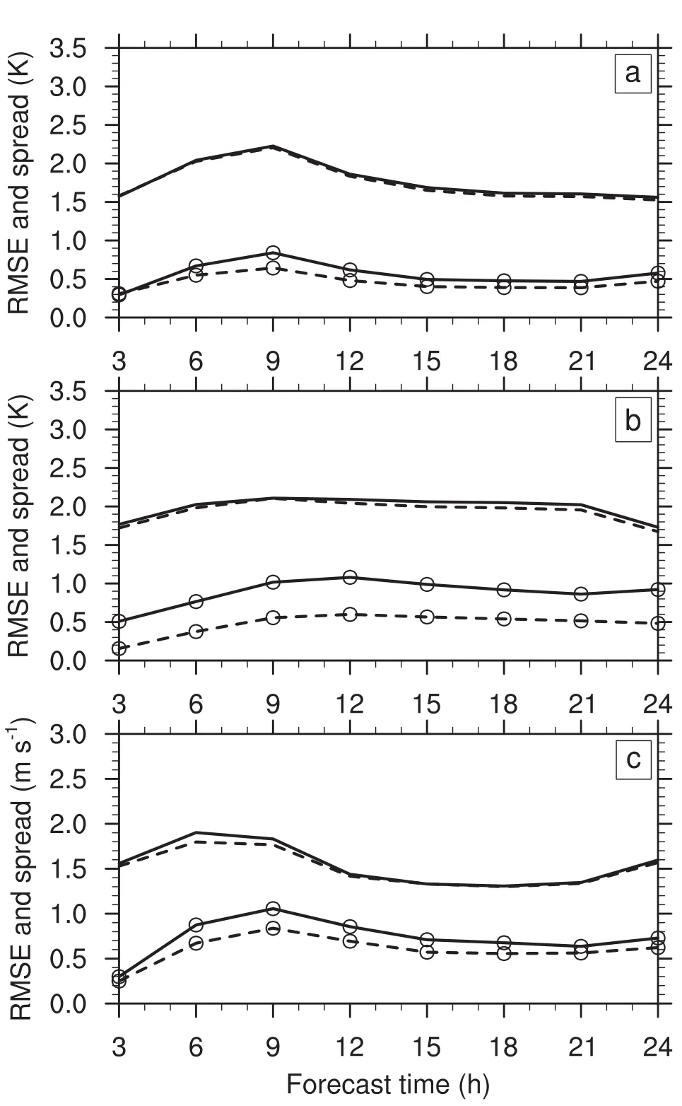
Fig.7.As in Fig.5 but for MPPE and ISMPE after bias removal.

The bias score for APCP24 shows that daily precipitation increased with ISM among the ensemble members.A wetter ISM,such as in ERA-Interim,produced larger bias scores for all thresholds,i.e.,more precipitation.This correlation demonstrates that the region is moisture-limited(Seneviratne et al.,2010).The convective available potential energy(CAPE)and convective inhibition(CIN)were verified for the five members of ISMPE on 11 days with the domainaveraged rainfall amount exceeding 5 mm,along with a time series of 1-h accumulated precipitation analysis averaged on all available days(Fig.12).Since precipitation has different characteristics over the plateau and plain in northern China(He and Zhang,2010),the veri fication was performed separately for these two areas.The 200-m terrain height contour line along the Yanshan and Taihang mountains was used to divide the 4-km domain into two parts,with the plateau on the left and plain on the right(thick line in Fig.1b).The 200-m height contour line was used instead of a lower height contour line to avoid including in the plateau small hilly areas on the plain.The time series of precipitation shows that both the plateau and plain areas had active afternoon convection precipitation during the two months(maxima at about 8 h,1600 LST),while there was considerable evening precipitation over the plain,which was probably a result of precipitation propagating from the plateau(He and Zhang,2010).Over the plateau,a wetter ISM tended to produce larger CAPE,but changed CIN little,during afternoon;whereas,over the plain,a wetter ISM produced larger CAPE,and less CIN.Therefore,a wetter ISM is more conducive to convection in both the plateau and plain areas in the 4-km domain.

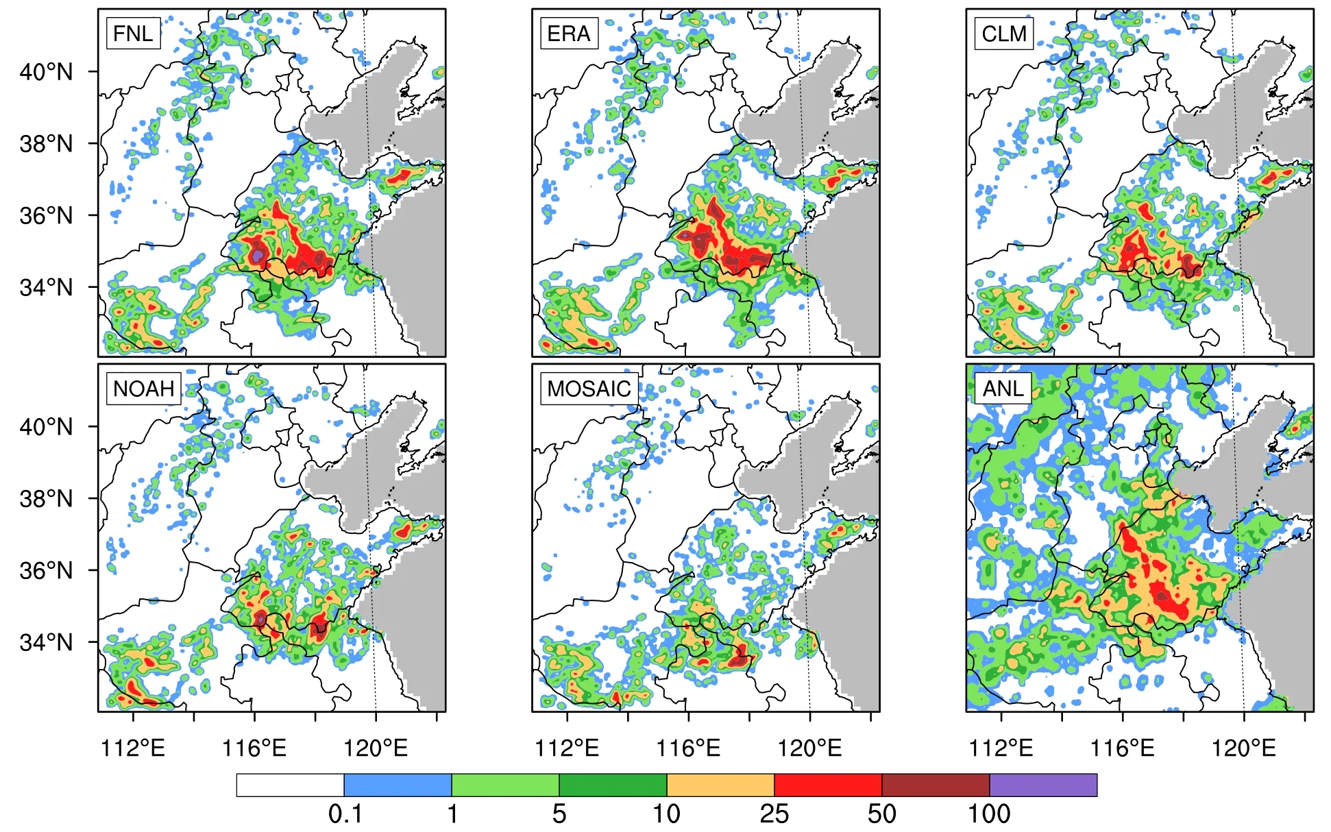
Fig.8.APCP24(mm)forecasts from the five members of ISMPE at 0000 UTC 14 July 2014,along with the corresponding rainfall analysis(ANL).The sea area is shown in grey.

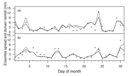
Fig.9.Ensemble spread of the APCP24 forecast of ISMPE(solid line)and MPPE(dashed line)in(a)July and(b)August 2014,along with the domain-averaged rainfall analysis(markers,missing on 15 July).

However,interactionbetweensoilmoistureandprecipitation may be complex at smaller scales.Many studies have reported negative feedback between soil moisture and convective precipitation.A wetter ISM may yield less vigorous thermals for convection initiation in convection-allowing NWP(Hohenegger et al.,2009).The wetter soil moisture may suppress storms by weakening cold pools due to less evaporation within the boundary layer(Van Weverberg et al.,2010).Some other studies have also reported negative feedback of soil moisture to convection,either through observation(Taylor and Ellis,2006)or numerical simulation(Quintanar and Mahmood,2012).Therefore,the interaction between soil moisture and precipitation on smaller spatial and temporal scales over this region is worthy of further study.

4.Summary

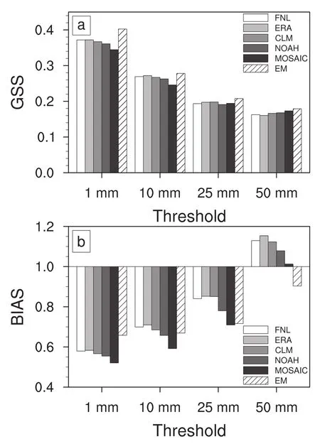
Fig.10.GSS and bias scores of the five members of ISMPE for thresholds of 1 mm,10 mm,25 mm and 50 mm.EM:ensemble mean.

Research into explicitly representing land surface uncertainties has been carried out for forecasts from short-range to climatic scales,providing promising results.To investigate the impact of ISM uncertainty on the ensemble spread and forecast skill of SREFs,we carried out an ISM-perturbed SREF experiment over a northern China domain for two summer months(July and August)in 2014.ISMPE consisted of a five-member forecast initiated with different soil moisture analyses produced by three research/operational centers.In addition,another five-member ensemble forecast con figured with mixed MP schemes was also performed for comparison with ISMPE.

ISM perturbation was shown to have notable effects on ensemble spread at the bottom and lower levels of the troposphere(below 800 hPa)in both daytime and nighttime,with the effects also propagating to higher levels of the atmosphere.The influence of the soil moisture perturbation was somewhat constrained to the lowest levels during nighttime because of surface cooling.Compared with MPPE,ISMPE produced larger ensemble spread below the middle troposphere(about 500 hPa).Thus,ISM uncertainty can have an important effect on atmospheric variables in northern China during summertime,which makes it a significant source of uncertainty in SREFs.

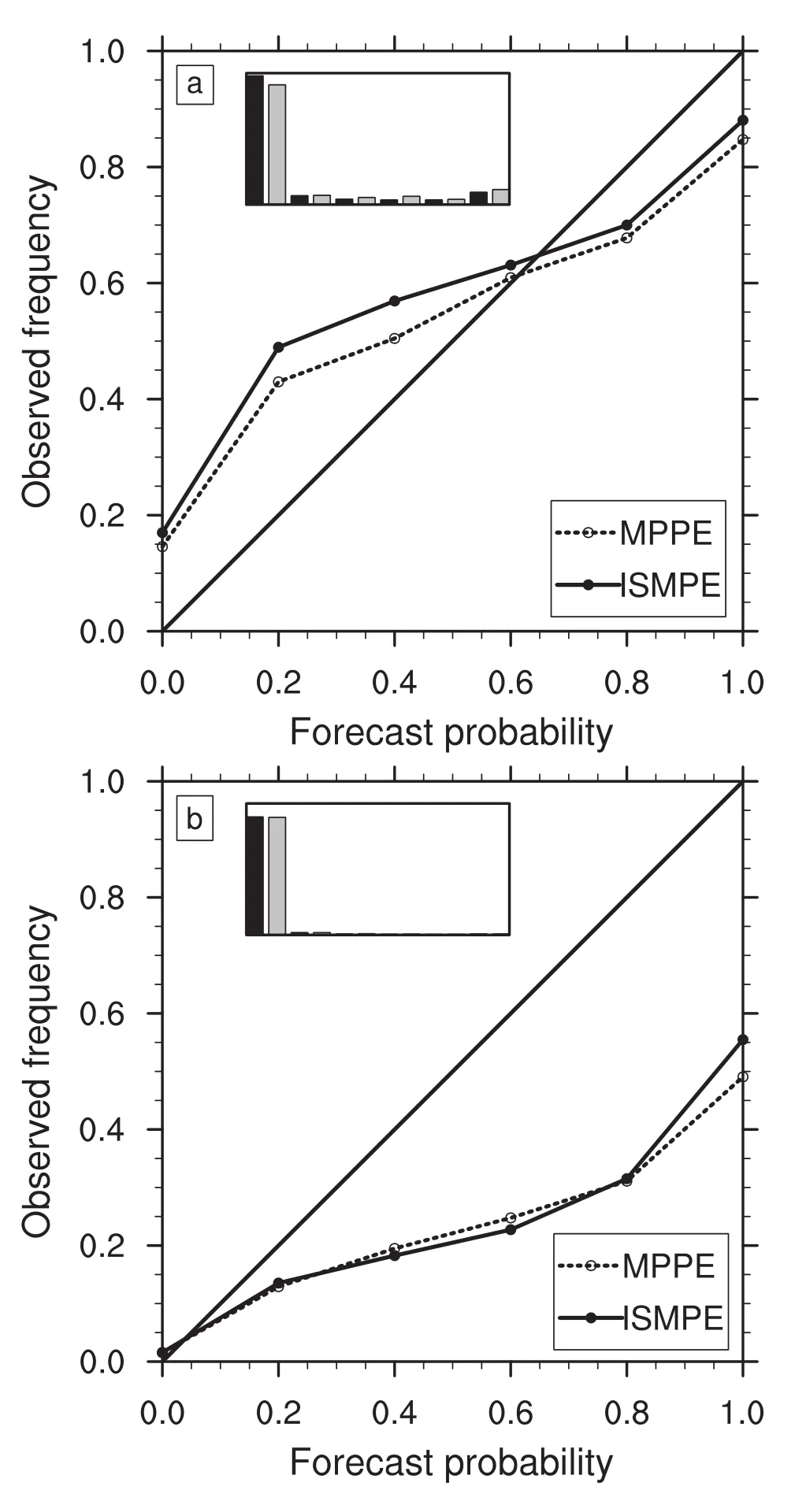
Fig.11.Reliability diagrams of probabilistic forecasts of ISMPE and MPPE for APCP24 exceeding(a)1 mm and(b)25 mm.The grey bar in the inset histogram is the frequency of the forecast probability of ISMPE,while the black bar is for MPPE.

ISM perturbation can increase the ensemble spread in near-surface variable forecasts.However,the increased ensemble spread contained contributions from both stochastic error growth and bias,of which only the former was useful.To remove the bias part from the ensemble spread,mean bias removal was performed for all forecasts.ISMPE still had larger ensemble spread than MPPE after bias removal,demonstrating that perturbing ISM is advantageous for representing stochastic error in near-surface variable forecasts.However,ISMPE was still under-dispersed at the near surface level,indicating the uncertainty cannot be fully represented by ISM perturbation alone.

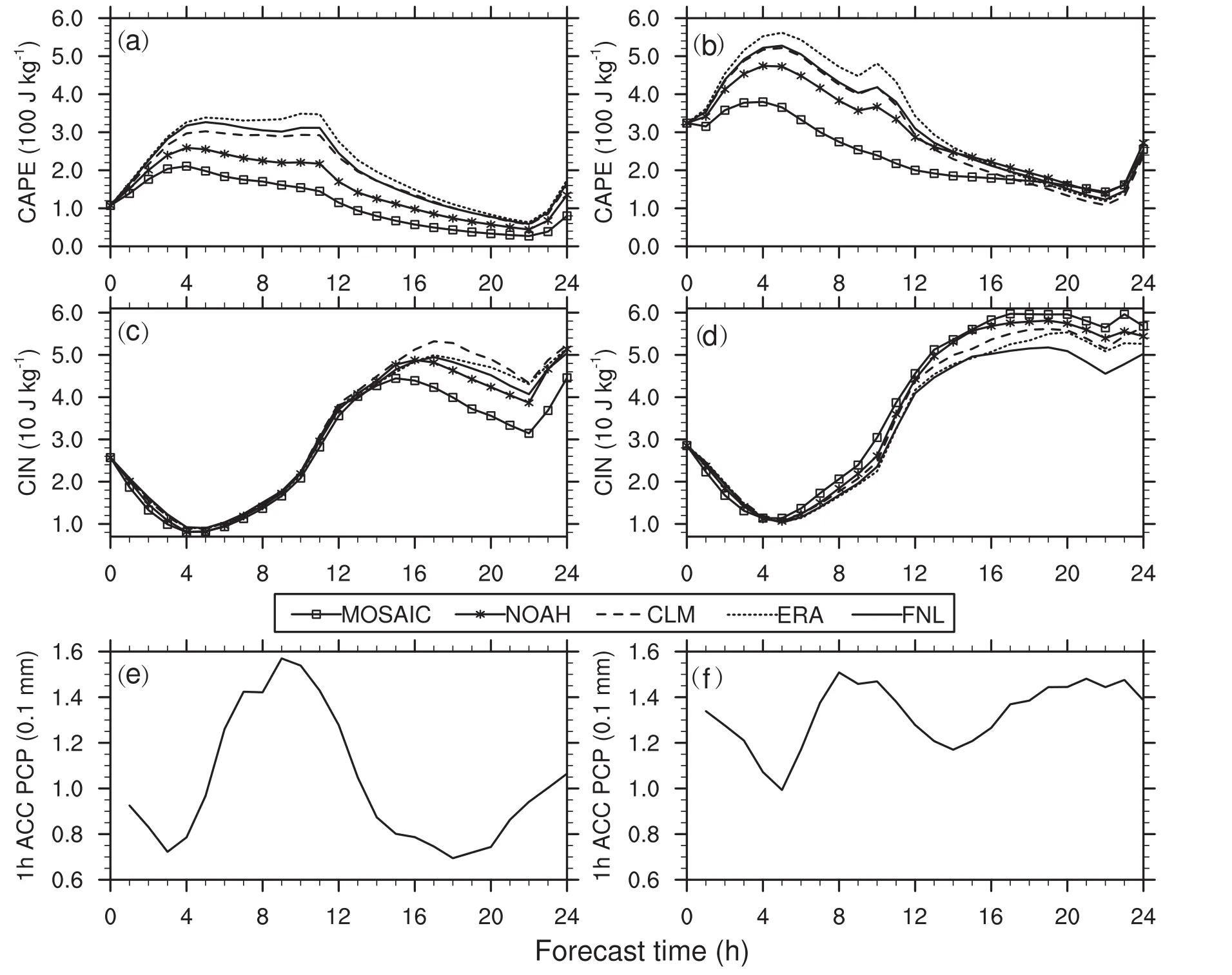
Fig.12.The(a,b)CAPE and(c,d)CIN of the five members of ISMPE,averaged on 11 days with domain-averaged rainfall exceeding 5 mm,and(e,f)time series of 1-h accumulated precipitation,averaged from 1 July to 31 August 2014,over the(a,c,e)plateau region and(b,d,f)plain region.

Perturbing ISM also had a notable influence on summertime daily precipitation forecasts over northern China.ISMPE produced slightly less but comparable ensemble spread to MPPE on most days,with the exception of several days with very strong synoptic forcing.ISMPE produced a skillful ensemble-mean precipitation forecast that outperformed any single ensemble member for all verification thresholds.ISMPE had a better BS and resolution than MPPE in probabilistic precipitation forecasts for thresholds of 10 mm,25 mm and 50 mm,showing its advantage in forecasting relatively larger precipitation amounts.A wetter ISM tends to produce a larger daily precipitation forecast over the domain.

In the present study we only carried out experiments for a two-month period in 2014,which did not include the impacts of soil moisture variations in different years,such as much wetter or dryer soil moisture initial conditions.Therefore,more experiments at larger sample sizes are needed in the future.Since ISMPE was under-dispersed,coupling the ISM perturbation with perturbed atmospheric fields and jointly presenting other land surface uncertainty sources is needed for a better ensemble spread at the near-surface level,which is worth studying in the future.Comparison with other land surface perturbation methods,such as breeding methods and parameter perturbation,is worth studying in future as well.

Acknowledgements.We thank the two anonymous reviewers for their valuable comments,which helped to improve this manuscript.The data used in this study were acquired as part of the mission of NASA’s Earth Science Division and archived and distributed by the Goddard Earth Sciences Data and Information Services Center.This research was jointly supported by the National Key R&D Program on Monitoring,Early Warning and Prevention of Major Natural Disaster(2017YFC1502103)and the National Natural Science Foundation of China(Grant Nos.41305099 and 41305053).

APPENDIX

The GSS and bias score were used to examine the skill of the precipitation forecast for rainfall amounts exceeding a particular threshold.The GSS measures how well forecast events match observed events,with reference to random chance.The GSS ranges from?1/3 to 1.A positive score indicates a forecast is better than a random forecast.The score is defined as

wherehis the number of hits,matches between a “Yes”forecast and a “Yes”observation;mthe number of misses,“No”forecasts with “Yes”observations;andfthe number of false alarms,“Yes”forecasts with “No”observations.Thehrterm refers to the number of random hits,defined as

wheretis the number of all verified forecast–observation pairs.

The bias score is a good supplement to the GSS.It measures whether a forecast overestimates(BIAS＞1)or underestimates(BIAS＜1)observed events,and is defined as

The BS was used to verify the probabilistic precipitation forecast for a particular threshold.It is the mean-squared error of the probabilistic forecast,in which a smaller value indicates a better performance.The score is defined as

wherepis the forecast probability,othe occurrence of the event,iis the index of sample points,andNis the total sample size.

By categorizing forecast sin toK(ensemblesize+1)probability bins,the BS can be decomposed into three terms:

wherek,nk,pkandokare the index,sample size,forecast probability and observed frequency,respectively,of the probability bins;andˉois the observed frequency of the overall sample.The first term is the reliability,which measures how well the forecasted probability matches the observed frequency(the smaller the value the better);the second is the resolution,which measures how well the forecast discriminates events of different probability(the larger the value the better);and the third is the uncertainty,which measures the variance of the observed event.When the ensemble size is relatively large,Kcan be set to a number less than the ensemble size+1,and Eq.(5)will hold approximately.

REFERENCES

Aligo,E.A.,W.A.GallusJr.,andM.Segal,2007:Summerrainfall forecast spread in an ensemble initialized with different soil moisture analyses.Wea.Forecasting,22,299–314,https://doi.org/10.1175/WAF995.1.

Case,J.L.,S.V.Kumar,J.Srikishen,and G.J.Jedlovec,2011:Improving numerical weather predictions of summertime precipitation over the southeastern united states through a highresolution initialization of the surface state.Wea.Forecasting,26,785–807,https://doi.org/10.1175/2011WAF2222455.1.

Chen,F.,andJ.Dudhia,2001:Coupling an advanced land surface––hydrology model with the Penn State–NCAR MM5 modeling system.Part I:Model implementation and sensitivity.Mon.Wea.Rev.,129,569–585,https://doi.org/10.1175/1520-0493(2001)129＜0569:CAALSH＞2.0.CO;2.

Chen,F.,and Y.Zhang,2009:On the coupling strength between the land surface and the atmosphere:From viewpoint of surface exchange coefficients.Geophys.Res.Lett.,36,L10404,https://doi.org/10.1029/2009GL037980.

Chen,S.,and Coauthors,2016:Precipitation spectra analysis over China with high-resolution measurements from optimally merged satellite/gauge observations—Part II:Diurnal variability analysis.IEEE Journal of Selected Topics in Applied Earth Observations and Remote Sensing,9,2979–2988,https://doi.org/10.1109/JSTARS.2016.2529001.

Chen,X.L.,X.S.Shen,and H.P.Chen,2010:Analysis of the impact of land surface process on numerical weather predication of intensive summer rainfall over Huai River in 2007.Journal of Tropical Meteorology,26,667–679,https://doi.org/10.3969/j.issn.1004-4965.2010.06.004.(in Chinese)

Cheng,F.-Y.,Y.-C.Hsu,P.-L.Lin,and T.-H.Lin,2013:Investigation of the effects of different land use and land cover patterns on mesoscale meteorological simulations in the Taiwan Area.J.Appl.Meteor.Climatol.,52,570–587,https://doi.org/10.1175/JAMC-D-12-0109.1.

Dee,D.P.,and Coauthors,2011:The ERA-Interim reanalysis:Con figuration and performance of the data assimilation system.Quart.J.Roy.Meteor.Soc.,137,553–597,https://doi.org/10.1002/qj.828.

Duda,J.D.,X.G.Wang,F.Y.Kong,and M.Xue,2014:Using varied microphysics to account for uncertainty in warmseason QPF in a convection-allowing ensemble.Mon.Wea.Rev.,142,2198–2219,https://doi.org/10.1175/MWR-D-13-00297.1.

Ebert,E.E.,2001:Ability of a poor Man’s ensemble to predict the probability and distribution of precipitation.Mon.Wea.Rev.,129,2461–2480,https://doi.org/10.1175/1520-0493(2001)129＜2461:AOAPMS＞2.0.CO;2.

Eckel,F.A.,and C.F.Mass,2005:Aspects of effective mesoscale,short-range ensemble forecasting.Wea.Forecasting,20,328–350,https://doi.org/10.1175/WAF843.1.

He,H.Z.,and F.Q.Zhang,2010:Diurnal variations of warm season precipitation over northern China.Mon.Wea.Rev.,138,1017–1025,https://doi.org/10.1175/2010MWR3356.1.

Hohenegger,C.,P.Brockhaus,C.S.Bretherton,and C.Sch¨ar,2009:The soil moisture–precipitation feedback in simulations with explicit and parameterized convection.J.Climate,22,5003–5020,https://doi.org/10.1175/2009JCLI2604.1.

Hong,S.-Y.,Y.Noh,and J.Dudhia,2006:A new vertical diffusion package with an explicit treatment of entrainment processes.Mon.Wea.Rev.,134,2318–2341,https://doi.org/10.1175/MWR3199.1.

Hou,D.C.,E.Kalnay,and K.K.Droegemeier,2001:Objective veri fication of the SAMEX’98 ensemble forecasts.Mon.Wea.Rev.,129,73–91,https://doi.org/10.1175/1520-0493(2001)129＜0073:OVOTSE＞2.0.CO;2.

Iacono,M.J.,J.S.Delamere,E.J.Mlawer,M.W.Shephard,S.A.Clough,and W.D.Collins,2008:Radiative forcing by longlived greenhouse gases:Calculations with the AER radiative transfer models.J.Geophys.Res.,113,D13103,https://doi.org/10.1029/2008JD009944.

Kain,J.S.,2004:The Kain–Fritsch convective parameterization:An update.J.Appl.Meteor.,43,170–181,https://doi.org/10.1175/1520-0450(2004)043＜0170:TKCPAU＞2.0.CO;2.

Koster,R.D.,and Coauthors,2004:Regions of strong coupling between soil moisture and precipitation.Science,305,1138–1140,https://doi.org/10.1126/science.1100217.

Lim,K.-S.S.,and S.-Y.Hong,2010:Development of an effective double-moment cloud microphysics scheme with prognostic cloud condensation nuclei(CCN)for weather and climate models.Mon.Wea.Rev.,138,1587–1612,https://doi.org/10.1175/2009MWR2968.1.

Ma,Y.Z.,C.G.Lu,and S.T.Gao,2012:The effects of different microphysical schemes in WRF on a heavy rainfall in North China during 18–19 August 2010.Chinese Journal of Atmospheric Sciences,36(4),835–850,https://doi.org/10.3878/j.issn.1006-9895.2011.11159.(in Chinese)

MacLeod,D.A.,H.L.Cloke,F.Pap pen berger,and A.Weisheimer,2016:Improved seasonal prediction of the hot summer of 2003 over Europe through better representation of uncertainty in the land surface.Quart.J.Roy.Meteor.Soc.,142,79–90,https://doi.org/10.1002/qj.2631.

Meng,W.G.,Y.X.Zhang,J.N.Li,G.F.Dai,H.R.Li,and Y.Y.Huang,2012:Sensitivity of mesoscale convective systems and associated heavy rainfall to soil moisture over South China.Journal of Tropical Meteorology,28,633–645,https://doi.org/10.3969/j.issn.1004-4965.2012.05.003.(in Chinese)

Milbrandt,J.A.,and M.K.Yau,2005:A multimoment bulk microphysics parameterization.Part I:Analysis of the role of the spectral shape parameter.J.Atmos.Sci.,62,3051–3064,https://doi.org/10.1175/JAS3534.1.

Morrison,H.,G.Thompson,and V.Tatars kii,2009:Impact of cloud microphysics on the development of trailing stratiform precipitation in a simulated squall line:Comparison of one and two-moment schemes.Mon.Wea.Rev.,137,991–1007,https://doi.org/10.1175/2008MWR2556.1.

Mullen,S.L.,and R.Buizza,2001:Quantitative precipitation fore casts over the United States by the ECMWF ensemble prediction system.Mon.Wea.Rev.,129,638–663,https://doi.org/10.1175/1520-0493(2001)129＜0638:QPFOTU＞2.0.CO;2.

Orth,R.,E.Dutra,and F.Pappenberger,2016:Improving weather predictability by including land surface model parameter uncertainty.Mon.Wea.Rev.,144,1551–1569,https://doi.org/10.1175/MWR-D-15-0283.1.

Pielke,R.A.,2001:Influence of the spatial distribution of vegetation and soils on the prediction of cumulus Convective rainfall.Rev.Geophys.,39,151–177,https://doi.org/10.1029/1999RG000072.

Quintanar,A.I.,and R.Mahmood,2012:Ensemble forecast spread induced by soil moisture changes over mid-south and neigh bouring mid-western region of the USA.Tellus A,64,17156,https://doi.org/10.3402/tellusa.v64i0.17156.

Rodell,M.,and Coauthors,2004:The global land data assimilation system.Bull.Amer.Meteor.Soc.,85,381–394,https://doi.org/10.1175/BAMS-85-3-381.

Segal,M.,and R.W.Arritt,1992:Nonclassical mesoscale circulations caused by surface sensible heat- flux gradients.Bull.Amer.Meteor.Soc.,73,1593–1604,https://doi.org/10.1175/1520-0477(1992)073＜1593:NMCCBS＞2.0.CO;2.

Seneviratne,S.I.,and Coauthors,2010:Investigating soil moisture–climate interactions in a changing climate:A review.Earth-Science Reviews,99,125–161,http://dx.doi.org/10.1016/j.earscirev.2010.02.004.

Shen,Y.,P.Zhao,Y.Pan,and J.J.Yu,2014:A high spatiotemporal gauge-satellite merged precipitation analysis over China.J.Geophys.Res.,119,3063–3075,https://doi.org/10.1002/2013JD020686.

Smirnova,T.G.,J.M.Brown,and S.G.Benjamin,1997:Performance of different soil model con figurations in simulating ground surface temperature and surface fluxes.Mon.Wea.Rev.,125,1870–1884,https://doi.org/10.1175/1520-0493(1997)125＜1870:PODSMC＞2.0.CO;2.

Stensrud,D.J.,and N.Yussouf,2003:Short-range ensemble predictions of 2-m temperature and dewpoint temperature over New England.Mon.Wea.Rev.,131,2510–2524,https://doi.org/10.1175/1520-0493(2003)131＜2510:SEPOMT＞2.0.CO;2.

Sutton,C.,T.M.Hamill,and T.T.Warner,2006:Will perturbing soil moisture improve warm-season ensemble forecasts?A proof of concept.Mon.Wea.Rev.,134,3174–3189,https://doi.org/10.1175/MWR3248.1.

Taylor,C.M.,and R.J.Ellis,2006:Satellite detection of soil moisture impacts on convection at the mesoscale.Geophys.Res.Lett.,33,https://doi.org/10.1029/2005GL025252.

Taylor,C.M.,D.J.Parker,and P.P.Harris,2007:An observational case study of mesoscale atmospheric circulations induced by soil moisture.Geophys.Res.Lett.,34,L15801,https://doi.org/10.1029/2007GL030572.

Tennant,W.,and S.Beare,2014:New schemes to perturb seasurface temperature and soil moisture content in MOGREPS.Quart.J.Roy.Meteor.Soc.,140,1150–1160,https://doi.org/10.1002/qj.2202.

Tewari,M.,and Coauthors,2004:Implementation and verification of the unified NOAH land-surface model in the WRF model.Proceedings of 20th Conference on Weather Analysis and Forecasting/16th Conference on Numerical Weather Prediction,Seattle,WA,American Meteorological Society,11–15.

Thompson,G.,P.R.Field,R.M.Rasmussen,and W.D.Hall,2008:Explicit forecasts of winter precipitation using an improved bulk microphysics scheme.Part II:Implementation of a new snow parameterization.Mon.Wea.Rev.,136,5095–5115,https://doi.org/10.1175/2008MWR2387.1.

Trier,S.B.,F.Chen,and K.W.Manning,2004:A study of convection initiation in a mesoscale model using high-resolution land surface initial conditions.Mon.Wea.Rev.,132,2954–2976,https://doi.org/10.1175/MWR2839.1.

Trier,S.B.,F.Chen,K.W.Manning,M.A.LeMone,and C.A.Davis,2008:Sensitivity of the PBL and precipitation in 12-Day simulations of warm-season convection using different land surface models and soil wetness conditions.Mon.Wea.Rev.,136,2321–2343,https://doi.org/10.1175/2007 MWR2289.1.

Trier,S.B.,M.A.LeMone,F.Chen,and K.W.Manning,2010:Effects of surface heat and moisture exchange on ARW-WRF warm-season precipitation forecasts over the Central United States.Wea.Forecasting,26,3–25,https://doi.org/10.1175/2010WAF2222426.1.

Van Weverberg,K.,N.P.M.van Lipzig,L.Delobbe,and D.Lauwaet,2010:Sensitivity of quantitative precipita-tion forecast to soil moisture initialization and microphysics parametrization.Quart.J.Roy.Meteor.Soc.,136,978–996,https://doi.org/10.1002/qj.611.

Wang,Y.,A.Kann,M.Bellus,J.Pailleux,and C.Wittmann,2010:A strategy for perturbing surface initial conditions in LAMEPS.Atmos.Sci.Lett.,11,108–113,https://doi.org/10.1002/asl.260.

Zeng,X.M.,B.Wang,Y.Zhang,S.Song,X.Huang,Y.Zheng,C.Chen,and G.Wang,2014:Sensitivity of high-temperature weather to initial soil moisture:A case study using the WRF model.Atmos.Chem.Phys.,14,9623–9639,https://doi.org/10.5194/acp-14-9623-2014.

Zhang,C.L.,S.G.Miao,Q.C.Li,and F.Chen,2007:Impacts of fine-resolution land use information of Beijing on a summer severe rainfall simulation.Chinese Journal of Geophysics,50,1373–1382,https://doi.org/10.3321/j.issn:0001-5733.2007.05.012.(in Chinese)

Zhu,Z.,andC.X.Shi,2014:Simulation and evaluation of CLDAS and GLDAS soil moisture data in China.Science Technology and Engineering,14,138–144.(in Chinese)

Zuo,Z.Y.,and R.H.Zhang,2009:Temporal and spatial features of the soil moisture in boreal spring in eastern China.Science in China Series D:Earth Sciences,52,269–278,https://doi.org/10.1007/s11430-009-0011-5.