Self-Tuning Asynchronous Filter for Linear Gaussian System and Applications
Wenjun Lv,Yu Kang,Senior Member,IEEE,and Yunbo Zhao,Senior Member,IEEE
Abstract—In this paper,optimal filtering problem for a class of linear Gaussian systems is studied.The system states are updated at a fast uniform sampling rate and the measurements are sampled at a slow uniform sampling rate.The updating rate of system states is several times the sampling rate of measurements and the multiple is constant.To solve the problem,we will propose a self-tuning asynchronous filter whose contributions are twofold.First,the optimal filter at the sampling times when the measurements are available is derived in the linear minimum variance sense.Furthermore,considering the variation of noise statistics,a regulator is introduced to adjust the filtering coefficients adaptively.The case studies of wheeled robot navigation system and air quality evaluation system will show the effectiveness and practicability in engineering.
I.INTRODUCTION
DUE to its conciseness which may facilitate solutions,the linear Gaussian system is a preferable model to describe many physical systems,especially in engineering field such as target tracking,robot navigation,and fault diagnosis[1].The Kalman filter has been proved to be an optimal filter for linear Gaussian systems for the filtering problem[2].Furthermore,based on the concept of the conventional Kalman filter,a variety of improved Kalman filters have been investigated to solve different practical problems[3]-[8].This paper is devoted to solve the optimal filtering problem for a class of linear Gaussian systems where the system states are updated at a fast uniform sampling rate and the measurements are sampled at a slow uniform sampling rate.The updating rate of system states is several times the sampling rate of measurements and the multiple is constant.In other words,there is currently no available measurement methods for systems whose states update during the period between two adjacent measurements.Therefore,the conventional Kalman filter is invalid for this case due to the asynchronism between system states updating and measurements sampling.
The proposed problem in this paper can be categorized as either a filtering problem of a special class of systems suffering the measurement dropouts or delays,or a multirate information fusion problem.The distributed H∞filtering problem for a class of discrete-time Takagi-Sugeno fuzzy systems was investigated in[9].Compared with the robustfilter,there is no doubt that the optimal filter is preferred.The optimal linear estimation problem for linear discretetime stochastic systems with multiple packet dropouts are well investigated in[10]-[12].For this kind of systems,they developed the optimal filter,predictor,and smoother,whose solutions are computed via a Riccati difference equation.Aiming at the communication delays,the optimal filtering problem for the networked systems containing multi-state Markovian transmission delay and one-step random communication delay were investigated[13],[14].These works were investigated under the occurrences of measurement dropouts and delays which can be modelled as a stochastic process.However,the measurements are usually timestamped,so the time instants when these uncertainties occur are determinable.As for the multi-rate sampling discrete system,optimal linearfilter was obtained in the sense of linear minimum variance[15],[16].But the state argumentation method will result in huge computational complexity.Although modelling without resorting to state argumentation method,the filtering accuracy is relatively low in that the system noises were ignored during the modelling[17],[18].In this paper,in order to solve the aforementioned problem,the optimal filter at the sampling time when the measurements are available is derived in the linear minimum variance sense.Furthermore,considering the variation of noise statistics,a regulator is introduced to adjust the filtering coefficients adaptively.
The proposed filter has a typical application in wheeled robot navigation systems.The external references are often used to correct the navigation system by means of global positioning system(GPS)or the other approaches which are time-consuming[19]-[21],such that they will suffer from the multi-rate issue.Another application of the proposed filter can be found in the air quality evaluation systems to estimate the street air pollutant concentration in real time,which is of great significance due to its dominance for government to make more effective control strategies to improve the atmospheric environment.The conventional method termed as model-based method and the emerging technology called mobile-sensing method can be combined to improve the performance based on their complementary characteristics,but in an asynchronous way[22]-[24].In this paper,we consider the application of the proposed filter design for these two practical systems.
The rest of the paper is organized as follows.Section II formulates the problem.Section III discusses the solution in detail.Section IV is composed of two case studies,i.e.,the wheeled robot navigation system and the air quality evaluation system.The paper is concluded in Section V.
II.PROBLEMSTATEMENT
Considering a linear Gaussian system described by the following linear stochastic difference equation

where F,G,Γ and H are known time-invariant matrices with proper dimensions,t=0,1,...,is the sampling time of system states,Nt is the sampling time of measurements(N is termed as synchronization coefficient),xt∈Rnare the system states,yt∈Rmare the measurements,ut∈Rpare the controls,and wt∈Rqand vt∈Rmare the system noise and measurement noise,respectively.
The following assumptions are needed.
Assumption 1:The noises are independent Gaussian white processes such that

where Q and R are variance matrices of wtand vt,respectively; δtτis the Kronecker delta function where t and τ are both sampling times,δtτ=1 if t= τ and δtτ=0 otherwise;E represents mathematical expectation and prime is for the transposition.
Assumption 2:The pairwise structure(F,H)are completely observable,that is,the observability matrix O=[H,HF,...,HFn-1]′is of full-rank where F=FN.
Assumption 3:The noise variance matrices Q and R are unknown and slowly changing.
Remark 1:According to Assumption 1,the system and measurement noises are assumed to be the independent Gaussian white processes.This is reasonable for some practical systems.It is well known that many random variables(RVs)in nature are actually the sum of many independent RVs.According to the fact that the sum of independent RVs tends to a Gaussian RV regardless of their probability distribution functions[25];this is why the noises are assumed to have Gaussian distribution.As for the independence assumption,the coloured noise can be modelled by a linear system with white noise as its input,indicating that the coloured noise can be “whitened”by state argumentation method.
The problem is to develop a linear minimum variance filterbased on the measurement set{y0,yN,y2N,...,y?t/N」N}where?t/N」is the largest integer not larger than t/N.
III.SELF-TUNINGASYNCHRONOUSFILTERING
The proposed filter is first discussed,followed by the noise variance estimator.
A.Improved Kalman Filter
The Kalman filter has been proved to be an optimal filter for linear Gaussian systems.It estimates the system states and then obtains feedback in the form of measurement,dividing the equations into two groups:predictor equation and corrector equation.The former is responsible for projecting forward the current state estimations and error covariance to obtain the priori estimations for the next time instant.The latter is responsible for the feedback,that is,incorporating a new measurement into the priori estimations to obtain an improved posteriori estimation.The process is repeated with the previous posteriori estimation used to predict the new priori estimation.Hence,the Kalman filter performs as a time-variant recursive optimal filter.
Suppose that{yNt,t=0,1,...}is obtained at time Nt,coupled with the optimal estimationNtof xNtwhich is the linear summation of{yNt,t=0,1,...}.For the next time instant without measurement,we have

which is an unbiased estimation.Define the estimation errorand its variancethen

which is essentially the predicted estimation error variance in the conventional Kalman filter.
During the period of{Nt+τ,τ=1,2,...,N-1},

with the estimation error variance of

At the time Nt+N when the measurement is available,we have


Algorithm 1 Asynchronous Kalman Filter(ASYNCKF)
The effect on filtering performance brought by N can be obtained by a simple analysis.The estimation error variance Ptwill increase continuously during the period without measurements,because there is no measurements to correct the estimation.Meanwhile,a larger N will result in a larger Q,and thus a larger Ptat t=0,N,2N,....Therefore,there is no doubt that the filter performs better with the decrease of N.
The ASYNCKF algorithm is a time-varying recursive filter implemented by calculating the optimal Kalman gain Ktat t=0,N,2N,...,which brings great computational complexity;especially for high-dimensional matrices.However,if Ktis converged to a constant matrix K as t→∞,the time-invariantfilter can be obtained via substituting Ktby K.This is only available if the process equation(1a)and measurement model(1b)are synchronized.
Considering the period without measurements of{Nt+τ,τ=1,2,...,N-1},

and then setting τ=N,the synchronization model of(1a)and(1b)can be derived as


where the matrix K is set as a null matrix at t/=0,N,2N,...and a non-zero matrix at t=0,N,2N,...whose value can be determined by solving the following equation set

It has been proven that the time-invariant filter will converge to the optimal time-variant Kalman filter with probability one,and therefore the convergence of the time-invariant form of ASYNCKF can be easily deduced[27].Note that we use the word “time-invariant”here to show the invariance of KNt;the Kalman Gain switches between two constant matrices instead of an infinite set.This greatly reduces the computational complexity,making the time-invariant form more applicable in practice in spite of its sub-optimality.
B.Noise Variance Estimator
The proposed regulator can be described as a noise variance estimatorandwhich are the linear functions over{yNt,t=0,1,2,...}.Rewriting(9a)yields

where q-1is the backward shift operator such that q-1xt+1=xt.Then

Substituting(13)into(9b)yields

and then using

where adj is adjoint matrix and det is the determinant,(14)becomes

Conducting the left-coprime factorization[28]on both sides,we have

where A(q-N),Bμ(q-N)and Bω(q-N)are polynomial matrices with the form of

with A0=I,B0=0.Let zNt=A(q-N)yNt-Bμ(q-N)μN(yùn)t,then

where zNtis the sum of two independent moving average processes,so zNtis another moving average process whose order is the same as that of the component process of higher order[29].
Define the correlation function ofzNtas Λ(i)=where i=0,1,2,...,and=max(i,Λ(i)/=0).Then


Substituting the estimationsandinto(22)yields

So the remaining work is to design the estimators for Λ(i),that is,.Furthermore,considering the variation of noise statistics,the estimatormust gradually discard the history data,and thus
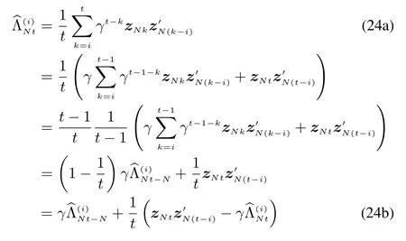
where 0<γ<1 is the fading factor whose fading rate grows as the positive number γ gets smaller.This is only available at Nt,t≥i while the estimation at other period can be determined by experience or arbitrarily for its asymptotical optimality.The γ should be selected as a larger number for slowly changing noises.To facilitate the implementation in computation,the recursive form is derived as shown in(24b).According to the ergodicity of stationary stochastic process we have→Λ(i)with probability one when t→∞.
The method in(24a)and(24b)is termed as the fading estimation.The alternative is the finite-memory estimation with the form of

whose recursive form does not exist.However,this method is still a promising solution.As seen in Fig.1,the blue plots represent for the weights assignment on history data of fading estimation,it is found that all the history data are shrunken sharply except the current one if γ is set to be a relatively small and positive.The fading factor is able to control the steepness of the blue plots.The finite-memory estimation shown as the red curve performs much better than that of the fading estimation in spite of the inexistence of recursive form.Hence,the fading estimation is favored in the real-time situation,and the finite-memory estimation is favored in the scenarios which require greater accuracy.
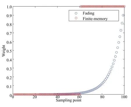
Fig.1.The comparison between fading estimation and finite-memory estimation on the weights assigned to the history data.
IV.CASESTUDIES
Two simulation tests for the wheeled robot navigation system and air quality evaluation system by applying the proposed self-tuning asynchronous filter will be presented.
A.Wheeled Robot Navigation System
A global positioning system(GPS)aided wheeled robot navigation system is composed of three parts:the space segment,the control segments and the user segment,as illustrated in Fig.2.The wheeled robot is mounted with a GPS receiver to determine its kinematic states.However,the GPS has a low updating frequency,and its signal may weaken due to various reasons.

Algorithm 2 Noise Variance Estimator(VAREST)
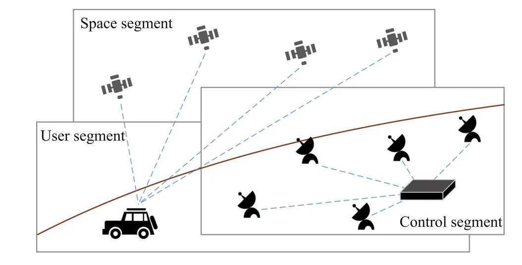
Fig.2.Illustration for wheeled robot navigation system.
The kinematics of a wheeled robot on roads can be approximately treated as the motion on the two-dimensional plane,which can be decomposed to the eastward motion and northward motion.Let T be the sampling time interval.The eastward motion is described by eastward location xE,tand eastward velocityat time Tt.Similarly,the northward motion is described by northward location xN,tand northward velocityat time Tt.Based on the Newton’s laws of motion,the eastward motion and northward motion are modelled as

where uE,t,uN,t,wE,tand wN,tare the eastward input acceleration,northward input acceleration,eastward random acceleration,and northward random acceleration,respectively.
They can be modelled as Gaussian white noises with changing variance.The updating rate of GPS is usually slower than that of uE,tand uN,tthus we have the measurement equation as

where yE,Ntand yN,Ntare eastward location and northward location derived from the GPS readings.The noise vE,Ntand vN,Ntmay change with time due to the influence brought by amount of observable satellites or interference signal.Similarly,they can be modelled as Gaussian white noises with changing variance.
Introducing the state variables xt=[xE,t,,xN,t,]′,yNt=[yE,Nt,yN,Nt]′,ut=[uE,t,uN,t]′,wt=[wE,t,wN,t]′and vNt=[vE,Nt,vN,Nt]′,the equations from(26a)to(26d),(27a)and(27b)can be rewritten in the form of(1a),(1b),(9a)and(9b)where
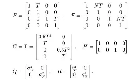
It is noted that the modelling procedure is very typical by applying some basic physical principles.It is also termed as the target tracking problem which is a popular research topic worldwide[27],[28].
Before the simulation,some parameters should be determined:the sampling time interval T=0.1,the noise variance=49 for the first half period and=900 for the second half period and=400 for the whole test.To verify the effectiveness of the proposed filter,three cases are taken into consideration as follows.
Case 1:The test is done using the asynchronous filter without considering the variation of noise characteristics.
Case 2:The test is done using the self-tuning asynchronousfilter.
Case 3:The test is done using the conventional Kalmanfilter.The last measurement received will be used to project forward the estimation while the measurements are missing.
The results are shown in Fig.3 where the black curves represent the real tracks and those in red,blue,and green for the estimations under different cases.The error is defined as the linear distance between the estimations and the real locations.The comparison between Case 1 and Case 2 indicates that the noise variance estimator is of significant importance for the influence brought by variation of noise characteristics can be eliminated to the largest extent.Using the last measurement to project forward the estimation can smooth the estimations during the period without measurements,but the comparison between Case 2 and Case 3 shows the superiority of the self-tuning asynchronous filter.Furthermore,the mean value of errors under the three cases are 54.74,39.54,and 72.03,respectively,such that the proposed filter has the smallest mean error.In summary,the proposed filter is relatively better than the existing methods.

Fig.3.Localization results and errors under the Cases 1,2 and 3.
Partially enlarging Fig.3(b)yields the Fig.4,where the blue circles represent measurements,the red curves are estimations,and the black curves are the real tracks.It is found that the data derived by dead-reckoning method without correction will diverge to infinity,but the GPS will correct the estimation in time while the error gets larger.Although the performance of dead-reckoning method deteriorates over time,it performs quite well in a short period,which has complemented the absence of GPS.Hence the wheeled robot navigation system is usually integrated with the two methods by fusing their outputs,to achieve a relatively accurate estimation in real time.
B.Air Quality Evaluation System
Based on the existing dispersion model shown in[30],[31],we will present a discrete linear parameterised box-type dispersion model,which is a parameterised semi-empirical model which makes use of a priori assumptions about the flow and dispersion conditions.As illustrated in Fig.5 the streets can be treated as a closed box with its top exchanging air with the high-level atmosphere for the very deepness of the street canyon.The inner atmosphere is relatively stable and the pollutant concentration will decrease with a fixed proportion k which is determined by the street structure.Due to the outmigration of high-pollution factories and the development in energy industry,traffic emission has become the dominant factor of street air pollution,especially in traffic-dense area.So it is assumed that the air pollution has arisen almost solely by traffic emission u.The high-level atmosphere is relatively stable such that its pollutant concentration is symbolized by a constant π.Hence,the atmospheric dispersion system can be described by

where xtis the street(the inner box)pollutant concentration,π the average high-level(the external box)pollutant concentration,utthe new concentration by traffic emission,wtthe Gaussian white noise,k∈(0,1)the dispersion coefficient and t the discrete time.The equation reveals how the inner-external differential concentration changes over time.Considering the uncertainty existing in the model,a Gaussian white noise wtis introduced to improve its precision.
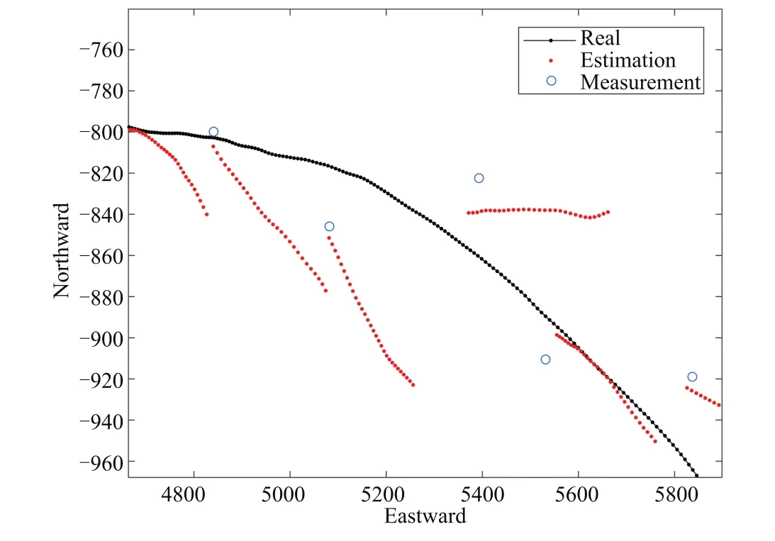
Fig.4.Partially enlarged detail in the Fig.3(b).
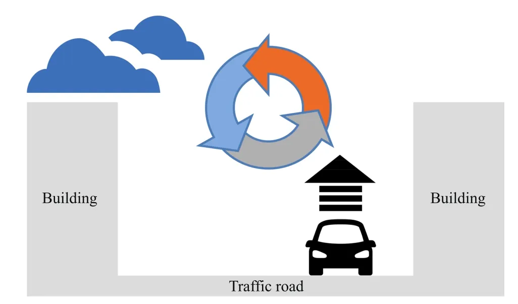
Fig.5.Illustration for atmospheric dispersion system.
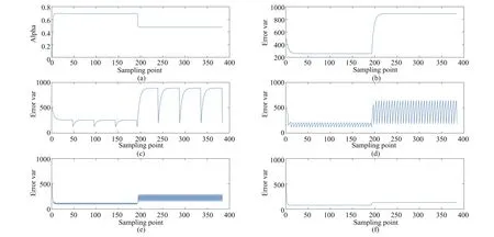
Fig.6.Simulation results for αtat t=0,N,2N,...and the estimation error variance under different N.
The monitoring cars equipped with atmospheric sensors can be used to correct the estimation.Rearranging(28)and modeling the mobile-sensing method yields

where χ =(1-k)π,ytstands for the outputs of monitoring car,wt~N(0,q),and vt~N(0,r)stand for two independent Gaussian white noises.The constant χ can be seen as the timeinvariant part of utsuch that this model is consistent with 1(a)and 1(b).
Set the parameters as dispersion coefficient k=0.8,noise variance q=49 for the first half period,q=169 for the second half period and r=250 for the whole test.In this test,the variation of estimation error variance under different N can be observed.It may give us a better understanding of the influence of accuracy by multi-rate-induced asynchronism.
The results are shown in Fig.6.The first test result in(a)shows the asymptotical stability,where the weight αtis set to be 0 initially and then converges to 0.6917 and 0.4761.It is found that the filter assigns more weights to the measurements with the increase of Q.Test results from(b)to(f)show the estimation error variance changing curve over time with different sampling time of measurements.The curves(b)show the estimation error variance with setting N as∞,that is,there is no available measurements during the whole test.However,the error does not go to infinity,but stays steady at 257.9 and 889.5 because the system itself is stable.The curves from(c)to(e)are based on setting N as 48,12 and 3,their error bounds are[126.9,257.9],[116.4,208.6],[93.85,125]for the first half period and[195.1,889.5],[183.5,643.3],[155,294.5]for the second half period,respectively.The filter seems to reduce the estimation error variance while it is getting large such that the upper bound can be significantly reduced before the variance reaches steady state.With the sampling time of measurements getting smaller,the upper bound of error is reduced at the same time.
V.CONCLUSION
In this paper,the optimal filtering problem for linear Gaussian systems is considered.A self-tuning asynchronous filter is proposed whose noise variance estimator is able to adjustfiltering coefficients adaptively.Two case studies,the wheeled robot navigation system and the air quality evaluation system,have demonstrated the effectiveness of the proposed approach.
 IEEE/CAA Journal of Automatica Sinica2018年6期
- IEEE/CAA Journal of Automatica Sinica的其它文章
- Predictive Tracking Control of Network-Based Agents With Communication Delays
- Speed-assigned Position Tracking Control of SRM With Adaptive Backstepping Control
- The Cubic Trigonometric Automatic Interpolation Spline
- Mathematical Study of A Memory Induced Biochemical System
- Optimal Decoupling Control Method and Its Application to a Ball Mill Coal-pulverizing System
- Necessary and Sufficient Conditions for Consensus in Third Order Multi-Agent Systems
