Parham M. Kebria,, Abbas Khosravi,, Syed Moshfeq Salaken, and Saeid Nahavandi, Senior

Abstract — Providing autonomous systems with an effective quantity and quality of information from a desired task is challenging. In particular, autonomous vehicles, must have a reliable vision of their workspace to robustly accomplish driving functions. Speaking of machine vision, deep learning techniques, and specifically convolutional neural networks, have been proven to be the state of the art technology in the field. As these networks typically involve millions of parameters and elements, designing an optimal architecture for deep learning structures is a difficult task which is globally under investigation by researchers. This study experimentally evaluates the impact of three major architectural properties of convolutional networks, including the number of layers, filters, and filter size on their performance. In this study, several models with different properties are developed,equally trained, and then applied to an autonomous car in a realistic simulation environment. A new ensemble approach is also proposed to calculate and update weights for the models regarding their mean squared error values. Based on design properties,performance results are reported and compared for further investigations. Surprisingly, the number of filters itself does not largely affect the performance efficiency. As a result, proper allocation of filters with different kernel sizes through the layers introduces a considerable improvement in the performance.Achievements of this study will provide the researchers with a clear clue and direction in designing optimal network architectures for deep learning purposes.

I. INTRODUCTION

INCREASING demand for autonomous systems requires a practical decision maker that guarantees their performance.In particular, autonomous vehicles require reliability of vision to be aware of the working environment. Moreover, costs and time spent on collection and preparation of useful data, and then training efforts are critical objectives in nowadays realworld applications. Sometimes results are not applicable for practical purposes and require more data and training to improve the performance. Deep neural networks, and specifically, convolutional neural networks (CNN) have demonstrated their impressive capability in processing large-scale image and video data [1]-[12]. A recent solution to deal with those expenses is imitation learning [13], [14]. Also known as learning from demonstration, it introduces a framework for a learning machine in which the machine learns how to perform a specific task by only observing (being fed by training data directly from) the human behaviour. This phase is so called demonstration [15]. Once the machine learns, it can then execute the same task by just mimicking what it has observed from a human operator [16].

Compared to other learning approaches, imitation learning is easier and more efficient in terms of computations and the amount of expert knowledge required for training process[16], [17]. Furthermore, it neither requires any explicit programming, nor heavily-proven mathematical analyses. In reinforcement learning techniques, for example, design of a reward-punishment function is necessary, which is sometimes a challenging task [16]. On the other side, thanks to the advancements in measurement technologies, a great value of sensory information is now provided, including visual,thermal, geometrical, and many other characteristic features of working environments. Thence, computers are able to easily process the collected data and generate the desired decision commands for a given task.

Imitation strategies are being widely used in autonomous systems. Simple in implementation and adaptable with many other learning techniques, imitation methods are gaining a great deal of attention in intelligent applications. Learning from demonstration considerably relaxes the assumptions and restrictions in applications where real-time perception of a desired task is a must. In reinforcement learning methods, for instance, investigation in an applicable and generalisable reward function might become practically difficult in fastresponse and time-critical applications, such as autonomous vehicles [18]-[21]. On the other hand, an imitation approach has its own challenges as well, where the learning algorithm should be carefully designed to generate robust and effective models. To cope with this concern, researchers have usually developed imitation methods incorporated with other intelligent algorithms, including deep learning [22]-[24],reinforcement learning [25], deep reinforcement learning [26],parallel reinforcement learning [27], supervised methods [28],and many others [29]-[31].

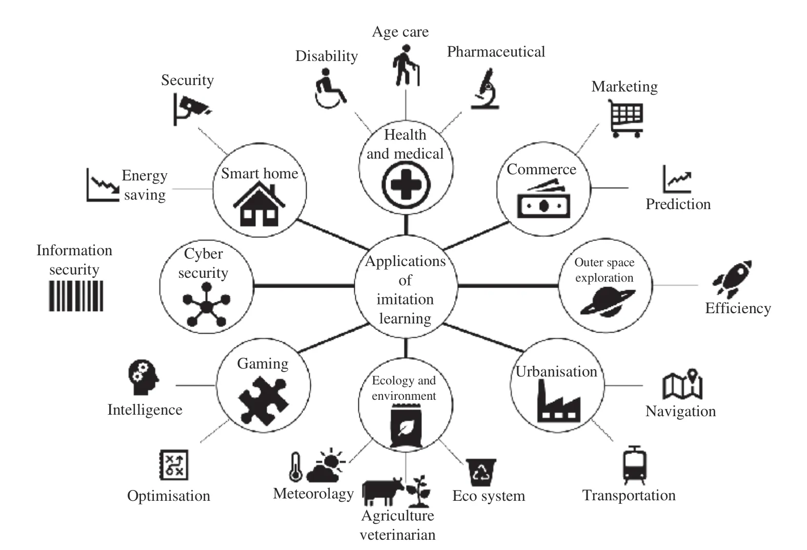
Fig. 1. Various applications of imitation learning.

Flexibility of imitation learning approaches also makes them to be easily developed for a variety of applications. As shown in Fig. 1, these applications include robotics [22], [32],autonomous systems [28], [33], unmanned vehicles [34], [35],automotive control [36], and computational games [37]. The common concept in every application of imitation learning is demonstration of a desired task performed by a human operator (expert knowledge). This can be achieved by a human driver, pilot, chief, etc. The required information might be collected by cameras, sensors, and any proper data acquisition tools. For example, in the case of autonomous vehicles either cameras or distance measurement sensors (e.g.infra-red) may be used for providing the vehicle with the road profile and environmental characteristics for training purposes.

Vision-based learning is one of the principle methods to teach a machine how to perform a given task [22], [28], [38],[39]. This is because when a machine is empowered by a vision tool, it can, to some extent, understand its surrounding environment, such as distances, obstacles, and shapes.Therefore, it is easier for the machine to learn how to avoid obstacles, using LIDAR [40], for example. On the other side,deep CNN algorithms are capable of processing visual data[41]-[47] very efficiently. Researchers have developed deep CNN structures to assess the influences of CNN structural parameters on performance of the output models. Several deep CNN configurations have been examined over a large-scale image dataset to evaluate the impact of the depth of CNN on output accuracy [5], [38]. However, finding the optimal depth of the network is still an active research question. In addition,the effect of the number and size of the convolutional filters(channel and kernel) in each layer on the output performance and transferability of layers is yet to be fully investigated [48].This has motivated us to develop several CNN models with architectures different in complexities: depth, number of filters, and filter size. Comparing the resulting performance of each model against well-known criteria, like mean squared error (MSE), this research gives an informative insight into CNN performance characteristics for imitation learning in autonomous driving scenario.

The main contributions of this article are:

1) A comprehensive evaluation and comparison of the three major architectural parameters, including the number of layers, filters, and kernel size in the design of a CNN, and their impact on the network’s overall performance. This comparison gives the researchers an overview of the most effective way to optimally design their deep networks to achieve the best possible performance.

2) A new MSE-based ensemble methodology for regression problems that improves the performance according to the average performance of each model throughout the previous observation samples.

3) As a popular ensemble approach, Bagging method is also considered to comparatively illustrate the superiority of the proposed ensemble approach.

4) Demonstrative comparison between the developed models provides the information about the impact of design parameters on the overall performance which leads to optimal structures for better performances.

To achieve this goal, the demonstration phase of a learning process is executed by a human driving a car in a simulation workspace. Three cameras on the vehicle continuously capture images from front, right, and left views from the car, while the human operator is driving it. All images are then fed into a deep CNN for processing and model generation. CNN outputs the desired steering angle as a decision command. Expectation of this process is to generate a model from only the images taken by the cameras. The generated model is expected to drive the car autonomously. To evaluate the performance of the resulting models, this study considers the impacts of quantity and size of the convolutional layers of each model.To this end, several models are developed with different structures in terms of the number of convolutional layers,number of convolutional filters (channels) in each layer, and filters’ size. It should be mentioned that all models are trained by the same training dataset, and then, tested over an identical input data. Furthermore, a new ensemble approach is proposed that calculates and updates weights for each model based on its MSE value. Having said that, this study develops a deep imitation learning methodology for an autonomous vehicle.Also, it provides a comprehensive evaluation study on structural properties of deep CNN models and their impacts on performance of the autonomous vehicle driving.

Fig. 2. The scheme of a typical convolutional neural network (CNN).

Rest of the paper is organised as follows. Section II describes a model development, the proposed ensemble approach, and training methodology. Experimental simulations for data collection and demonstration are presented in Section III. Then, Section IV discusses on the results, followed by conclusions and future directions in Sections V and VI, respectively.

II. PROPOSED METHODOLOGY

This section presents a methodology for CNN-based model development and the process of learning from demonstration.First, we briefly describe the CNN architectures developed in this paper for image processing purposes. The procedure of a learning policy by observing a human operator is then explained.

A. Convolutional Neural Network

As a kind of deep artificial neural networks, CNN has found a broad range of applications in computer vision and natural language processing [3]-[7]. CNN is one of the strongest tools in image classification, and therefore, in machine learning applications. In the case of autonomous vehicles, CNN models are also utilised for providing them with a visual sense and perception of their environment. CNN configurations enjoy from scattered connections and sharing weights. Depth in the context of CNN refers to the number of convolutional layers;the more the layers, the deeper CNN. Each layer has its own features and properties, including the number and size of convolutional filters (kernels). A deep CNN enforces local connections among neighbour neurons, which results in spatial correlations through the network. Fig. 2 shows the schematic of a typical CNN.

In this study, we develop and apply several CNN models with different architectures to evaluate their efficiency and effectiveness on the performance of an autonomous vehicle.We start from the shallowest and simplest architecture with 3 convolutional layers, 4 filters with the size of 3×3, and then gradually increasing their depth and complexity to 18 layers,32 filters, and filter size up to 7×7. It should be mentioned that the selected numbers are chosen according to the previous studies [5]. We also develop several models in which filter size changes after each max-pooling, i.e., 7×7 in the first layers, 5×5 after the first max-pooling, and 3×3 after the next and final max-pooling. Comparison of the outcomes of these models with that of the models with fixed filter size tends to illustrate the effect of filter size on overall performance.Notably, the number of filters are only indicated for the first convolutional layer in each model. Thence, the number of convolutional filters is doubled after every max-pooling. In total, 96 CNN models are developed with different configurations. In this regard, we assign a 3-digit ID for every model to show its structural properties. For instance, the model ID “1Convf×s” means that the corresponding model has 1 convolutional layers,ffilters in the first layer, ands×sfilter size, respectively. Additionally, the models with different filter size are identified as “1Convf×S_s” with filter sizeS×Sin the first layers, shrinking down tos×sin the last layers. Moreover, all models have been ended up by an identical, fully-connected dense layer consisting of 100×50×10×1 nodes. Table I presents the structural properties of the CNN models developed and applied in this study.Thereafter, we only use models’ ID for referring to a particular model.

B. Proposed Ensemble Approach

For further investigations and improvements in performance of CNN models here we propose and apply an ensemble approach. Ensemble formalisation for regression problems had been extensively studied in [49]. Therefore, here we briefly present the concept. Consideringas output of the modellC onvfs(andforlC onvfS_s) , andy?as the desired output (steering angle), then MSE of each model at sampling timetk＞0 is calculated as:

and the ensemble output forNmodels is generally considered as:

in which,wiis weight of theit h model with the outputyi, andNis the total number of models considered in ensemble. In our case, weights are calculated based on MSE of the corresponding model. Henceforth, we introduce weights as:

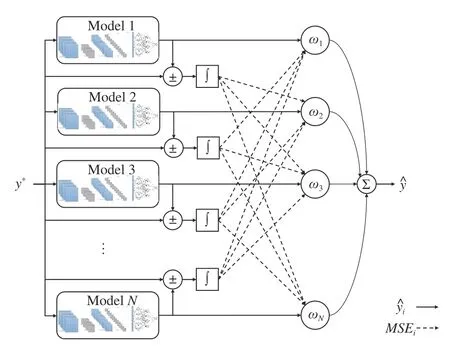
Fig. 3. Framework of the proposed MSE-based ensemble approach.

where numerator of the fraction in (3) is summation of all models’ MSE value excluding the corresponding modelthat the weight is being calculated for. Moreover, the denominator in (3) is summation of MSE of theNmodels considered in the ensemble:

Therefore (3) can be simplified as:

The reason for the multiplier (N-1) in the denominator in(4) is to satisfy the conditions in (2). To show this, adding all weights together results in:

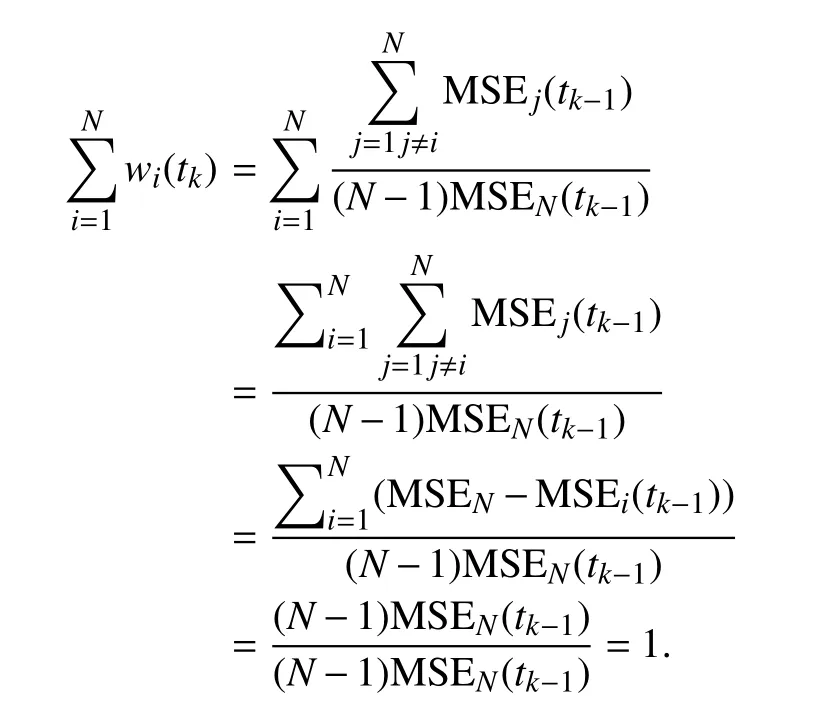
Additionally, at every sampling timetkweights are being derived based on MSE from previous sampling timetk-1. This way, weights are being updated regarding the recent values of MSE of the corresponding model and, notably, models that recently had less MSE value will have more contribution in the ensemble output. The workflow of the proposed MSEbased ensemble approach is illustrated in Fig. 3. Furthermore,Section IV will argue and discuss the performance of all models, including the proposed ensemble approaches. As one of the most applied ensemble techniques for regression problems [50]-[53], bagging ensemble is also applied and compared to the proposed ensemble strategy in this paper.

C. Learning From Demonstration

For the demonstration purpose, we have collected photos of three different views from a human driver’s perspective. Once the human drivers are happy with their performance, the captured photos are recorded, and then, used for the imitation learning. It is worth mentioning that here we feed the CNN models with exactly the same raw photos captured by the cameras during simulation experiments. In this case, 14 412 images have been captured by the size of 320×160 pixels.Moreover, 80% of the photos have been used for the training and 20% for the test. The CNN models have to predict the best steering angle. Hence, every trained model is desired to output an acceptable steering angle, while the speed and acceleration of the vehicle are prescribed, for simplicity. More details of the training and simulations are presented in the next section.

III. EXPERIMENTAL RESULTS AND DISCUSSIONS

In this section, we describe the experimental setup and simulation considered for training an autonomous vehicle from demonstration. As previously mentioned, we utilise a simulation environment to collect the training data for the demonstration phase in a cost-effective way (Fig. 4). For this purpose, we have executed our experiments in a self-drivingcar simulator developed by Udacity [54]. The main advantage of this simulation environment is its capability of generating datasets suitable for offline supervised learning algorithms. To this aim, we have performed the following steps:

Fig. 4. Random sample photos taken by the cameras on the car.

1) The required training data for imitation learning are being collected while a human drives the car. In other words, three cameras have been considered on the car in a simulation environment. Every camera takes photos from the designated angle; left, right, and front views, respectively. Fig. 4 illustrates a random set of the photos taken by the cameras.These cameras constantly capture the images with the recording time samples.

2) After data collection, next step is to utilise the data for training the CNN models. CNN parameters are being updated by gradient descent algorithms. The models learn the control policy by imitation, similar to the original idea of “pixel to action”[55].

3) All images (Fig. 4) are in the size of 320 160 pixels.They are stored and labelled by time-instance and angle: left,front, or right. However, through the learning process they are fed into the models in no particular order. In total, 14,412 images have been captured as the dataset for a training procedure. Further details of the training properties are provided in Table II.

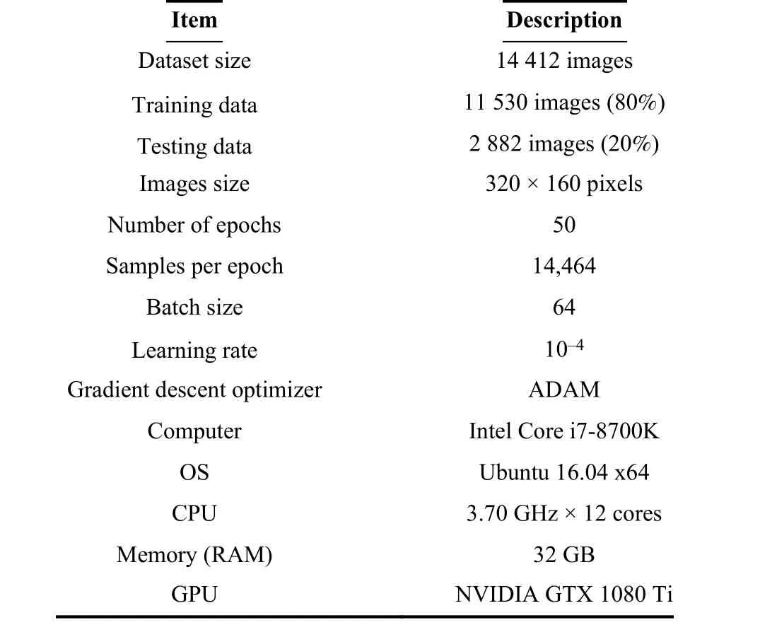
TABLE II TRAINING PARAMETERS AND PROPERTIES

4) To prevent over-fitting due to an imbalanced dataset, we forced the generator to augment images in real-time, while the models are being trained. We have provided the models with an equal chance of seeing different steering angles. Thence,we have reshaped the training data into their appropriate batches and trained the models at the same time.

5) In this step, several CNN models have been developed and trained. To have a better comparison and overview on effects of the architectural properties of each model on the final performance, models are developed with different structures (Table I). In other words, the number of layers(depth), the number of filters (channels), and filter size(kernels) increase by following a similar pattern. For validation, models are being tested on 20% of the data. Once all models have been trained and tested, they are evaluated on an autonomous vehicle for experimental performance examination and efficiency analyses.

It should be mentioned that the images are captured over three complete laps driven by the human driver. Although it is possible to collect more data by driving more laps, the aim of this study is to provide the learning agent with the minimum amount of data to decrease the effort and demonstration time.Also, it is worth to examine the developed learning methodologies under minimal data. Furthermore, collecting a great deal of data from different drivers with various driving styles, and in variety of driving conditions (weather, road profile, etc.) might be helpful for training models for general applications.

In the following, we fully present and discuss the resulting performance of the developed CNN models trained in the previous section. For evaluating and comparing the model performance and efficiency, we examine the output of every model based on well-known criteria, including loss function value, the number of trained parameters (weights), and training time (computational costs) of each model. Table III summarises the resulting numbers for the benchmarks of each model. Figs. 5-11 demonstrate the results for all the 96 developed CNN models and the ensemble in this study.Notably, the considered loss function is mean square error.

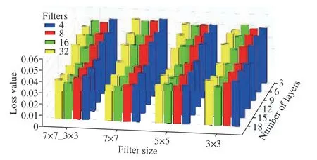
Fig. 5. Loss values (MSE) of the CNN models. This figure shows the filters size on the x axis and the number of layers on the y axis. Different colours indicate the number of filters. Moving along the y axis towards the deepest models, MSE decreases regardless of the number and size of the filters.Along the x axis, enlarging the filters results in lesser MSE. On the other hand, minimum error in every category chiefly happens among the models with 16 filters in the first layers (green bars).

As depicted in Fig. 5, moving from the back end of the figure towards the front end loss value of deeper models,specifically those with 12 layers and more, drops below 0.04.The most reduction occurs from 9Conv models to 12Conv ones. Although deeper models have resulted in less loss, the rate of reduction is not as large as that between 9 and 12 layers. Considering the quantity of filters, models with 16 and 32 filters in their first convolutional layers have shown a better performance. Surprisingly, in most of the configurations, models with 16 filters have slightly outperformed the more complicated models with 32 filters.This corollary is more visible in Fig. 9. Box plots of the loss values are illustrated with respect to different properties: (a)number of layers, (b) number of filters, and (c) the filter size.Also, Figs. 9 (d)-(f) show that the number of parameters significantly increases with respect to the quantity of layers and filters, while the size of filters has almost no impact on the number of parameters.

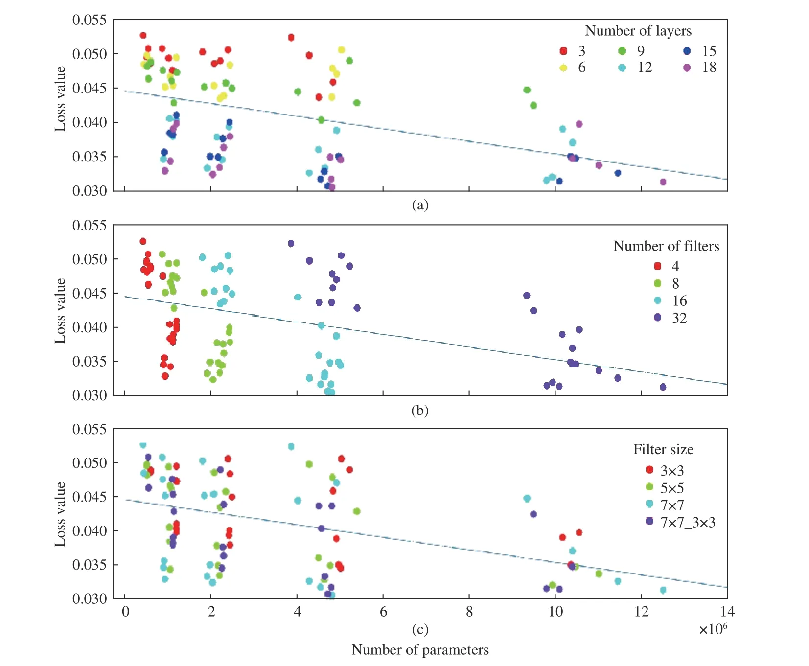
Fig. 6. Loss values of the CNN models and their trend line with respect to the number of parameters. In (a) colours indicate the number of layers. Deep models (light blue, dark blue, and purple) are mostly placed below the estimation line. Considering the horizontal axis, quantity of the layers does not increase the number of parameters as different colours are spread through that axis. In (b) models are coloured by their filters. Existence of all colours on either above and below the regressor line shows that the number of filters does not inevitably result in error reduction. Whilst, a monotone growing pattern is visible in the number of parameters due to increasing the number of filters. In (c), we can observe almost all colours in every region of the plot, which means that the size of filters has no momentous impact on the performance.

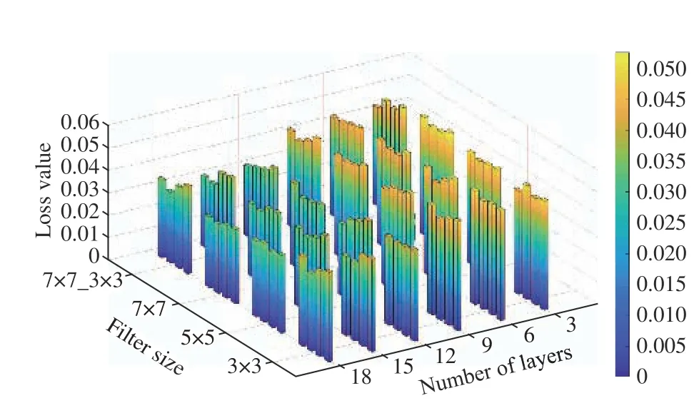
Fig. 7. Overall comparison of MSE values among the CNN models. It is apparent that the deeper models have less error. Moving from the right corner to the left corner of the graph, we see a big change in colours. In other words,deep models with bigger filters have outweighed the same-depth models with smaller filters.

Furthermore, Fig. 10 presents the growth in parameter count through the CNN models. Noticeably, models depth is sorted in the opposite direction of that of Fig. 5. As a result, the number of parameters increases as the models deepen.However, the growth in parameter count is more significant due to the number of filters (Figs. 9 and 10). On the other side,loss value decreases as the number of parameters increases.Fig. 6 shows the overall relation between the number of parameters and loss values, in three different presentations with respect to the configuration properties of the CNN models. Consequently, training time drastically increases as the number of parameters (Fig. 8). As it comes from Figs. 6 and 8, deeper models with 18 convolutional layers have the maximum parameter and training time, but the minimum loss value. Considering the computational cost and time, Fig. 8 compares the training time of the CNN models in terms of (a)the number of layers, (b) the number of filters, and (c) filter size, respectively. As it is shown in Fig. 8(b), models with the largest number of filters (32) lead to the great number of parameters and, subsequently, a great time of training. Whilst,Figs. 8(a) and (c) illustrate that even shallower models“9Conv” and smaller filters 5 × 5 and 3 × 3 take a considerable time for learning.

From Fig. 9, larger filters result in less errors. However,models with a mix of filter sizes have a better performance,and it shows that bigger filters only in the first layers can be more effective rather than enlarging filters throughout the network. Although size of the filters does not affect the total number of parameters (Fig. 9(f)), to some extent it reduces the computational cost as models with combined filter size 7 7_3 3have totally fewer parameters than those with the same number of layers and filters, but filters sized 7 × 7.Fig. 7 also shows the overall loss value of the models by scaling the colours, for better visualisations. The decreasing trend of the loss value among the models is quite apparent in it.

IV. CONCLUSIONS

Fig. 8. Training time of the CNN models and their trend line with respect to the number of parameters. Plot (a) groups the models in different colours based on the number of layers. Apparently, deeper models even with less parameters because of smaller filters, took a longer time to be trained. Similar to Fig. 6(b),here in (b) again we can see that models with more filters have substantially greater number of parameters, and therefore, longer training time. Scattered through plot (c), size of the filters neither did affect the number of parameters, nor the training time.

Having a reliable and robust vision is a mandatory requirement in autonomous vehicles, and convolutional neural networks are one of the most successful deep neural networks for image processing applications. On the other hand,applying imitation learning methods reduces the amount of training data, while speeding up the training process.However, CNN models generally require a great deal of training data and finding an optimal configuration for design parameters of a CNN is another challenge. In this paper, we consider an autonomous vehicle in a simulation environment and capture images from three different views from the car driven by a human, as the demonstration phase of imitation learning. The recorded data are then used for training CNN models. In this work, a total of 96 CNN architectures have been developed with a different number of layers, filters, and filter size, to investigate the impact of these three properties on the performance of CNN models.

The results show that the depth of the models causes a decrease the error (loss value). The minimum MSE achieved by the shallowest model (3 layers) is just below 0.045, while the maximum MSE by the deepest model (18 layers) is nearly 0.04. The biggest improvement is observed for models having layer counts between 9 and 12, where MSE drops from about 0.045 to 0.036. Additionally, utilising more filters in a network also reduces the error. The best results have been achieved by models having 16 filters in their first layers,though. In summary, increasing the number of filters does not necessarily result in a better performance. But the deeper models with larger filters in their first layers have an outstanding performance. As the results show, for this case study, a model with at least 12 layers, and 16 filters ranging from 7 × 7 in the first layers, to 3 × 3 through the last layers,has the best performance amongst the examined CNN architectures. However, finding the optimal architectural properties for a CNN is still under investigation. In this paper,we have analysed different structures for CNN to experimentally find a search range for the best architectural parameters.

Finally, we have proposed an ensemble approach which assigns weights for the models based on their recent MSE values. The proposed ensemble performed better than bagging; a well-known ensemble technique for regression problems. Applying an ensemble on different CNN models is recommended, as there might be various choices for design properties.

V. FUTURE WORK

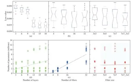
Fig. 9. (a) Shows box plots of the errors for every layer category. As shown in (b) the models with 16 filters have obtained the best results. Although error notably decreases due to an increase in the number of layers, a significant drop is observed between 9-layer and 12-layer models. As shown in (b) the models with 16 filters have obtained the best results. As illustrated in (c), having larger filters in the first layers, rather than throughout the network, results in a better performance. Considering two points on the regressor line in (e) with 16 and 32 values on the horizontal axis, and then comparing the corresponding numbers on the vertical axis, it is derived that the slope of the line is almost 1. As a result, growth in the number of parameters has approximately the same ratio as that of the number of filters. However, as (f) displays, enlarging the size of filters hardly affects the count of parameters. Moreover, taking into account the number of trainable parameters, the fitted regressor line in plot (e) has the steepest slope compared to (d) and (f).

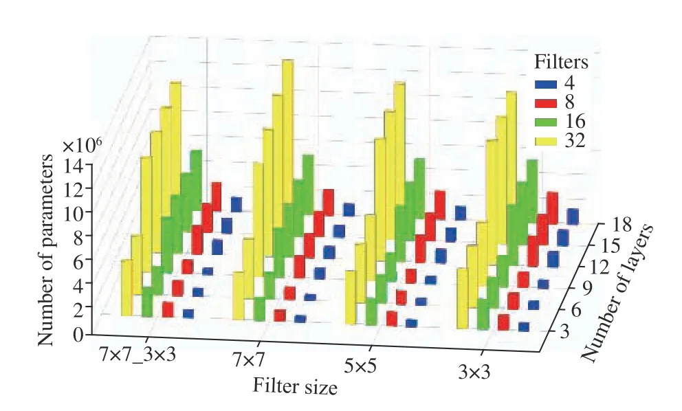
Fig. 10. Impact of design parameters on trainable parameters. As this figure shows, growth in the number of parameters is mostly caused by the quantity of filters in a CNN model. Models with more filters have a significantly larger number of parameters. Increasing the number of layers also leads to raise in the number of parameters, however, the size of filters does not have that distinguishable impact on parameters.

Although imitation CNN models have a promising outcome,the optimal design of a CNN for achieving the best performance is a highly demanded task in deep learning applications. Specifically, taking advantage of imitation learning methodologies requires the deep learning approaches to be as efficient as possible to make the whole process practically effective and robust. To achieve this goal, the optimal selection of parameters of the network and training procedure is an open question that researchers are actively investigating worldwide. The future of this research is to study more intelligent and efficient techniques, including genetic and evolutionary algorithms [56], [57] to obtain the optimum set of parameters.

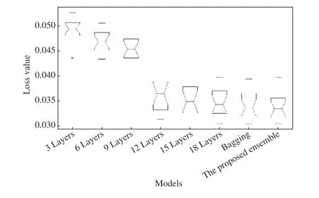
Fig. 11. Comparison between the models and ensembles. Bagging approach totally has a better performance due to its less medians. However, the proposed ensemble method not only outperforms all models, it also achieved a better result compared to the bagging technique. This happens because of upgrading the weights at every sample time based on the MSE values from previous samples.

APPENDIX

In this appendix, Table I demonstrates the structural and architectural properties of the CNN models developed in this study. Also, Table III presents the numerical results of the models performance, in terms of the number of trainable parameters, training time, and loss value (MSE).

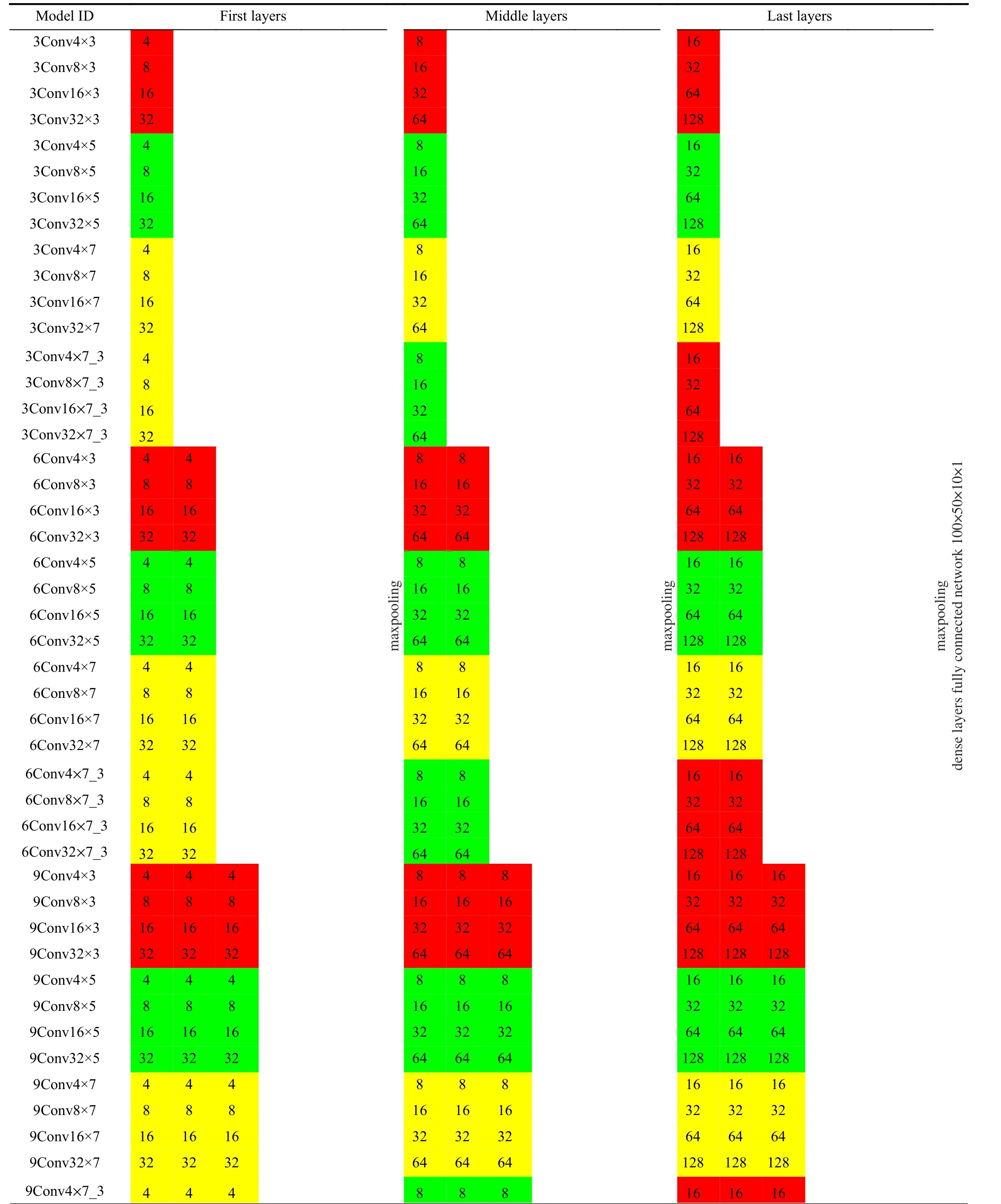
TABLE I STRUCTURAL PROPERTIES OF THE CNN MODELS. COLOURS RED, GREEN, AND YELLOW INDICATE THE FILTER SIZES 3 3, 5 5, AND 7 7,RESPECTIVELY. THE NUMBER IN EVERY COLOURED CELL PRESENTS THE COUNT OF FILTERS OF THE CORRESPONDING SIZE IN EACH LAYER

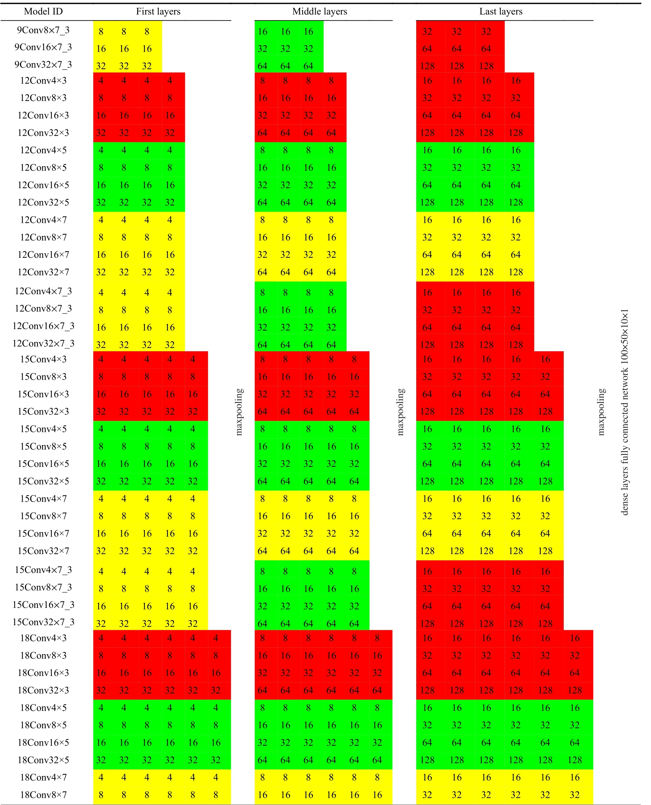
TABLE I (continued)STRUCTURAL PROPERTIES OF THE CNN MODELS. COLOURS RED, GREEN, AND YELLOW INDICATE THE FILTER SIZES 3 3, 5 5, AND 7 7,RESPECTIVELY. THE NUMBER IN EVERY COLOURED CELL PRESENTS THE COUNT OF FILTERS OF THE CORRESPONDING SIZE IN EACH LAYER

TABLE I (continued)STRUCTURAL PROPERTIES OF THE CNN MODELS. COLOURS RED, GREEN, AND YELLOW INDICATE THE FILTER SIZES 3 3, 5 5, AND 7 7,RESPECTIVELY. THE NUMBER IN EVERY COLOURED CELL PRESENTS THE COUNT OF FILTERS OF THE CORRESPONDING SIZE IN EACH LAYER

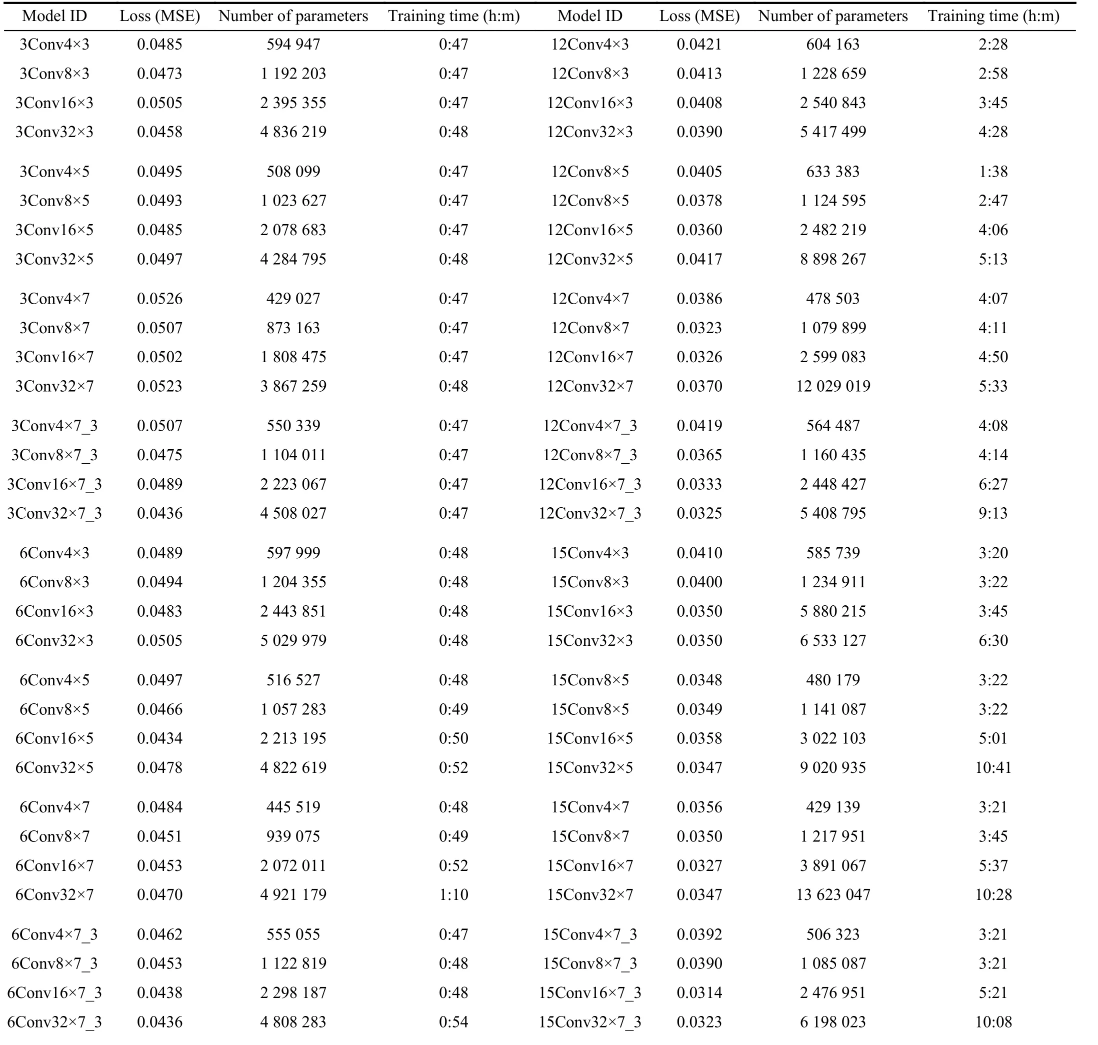
TABLE III NUMERICAL PERFORMANCE RESULTS OF THE TRAINED CNN MODELS

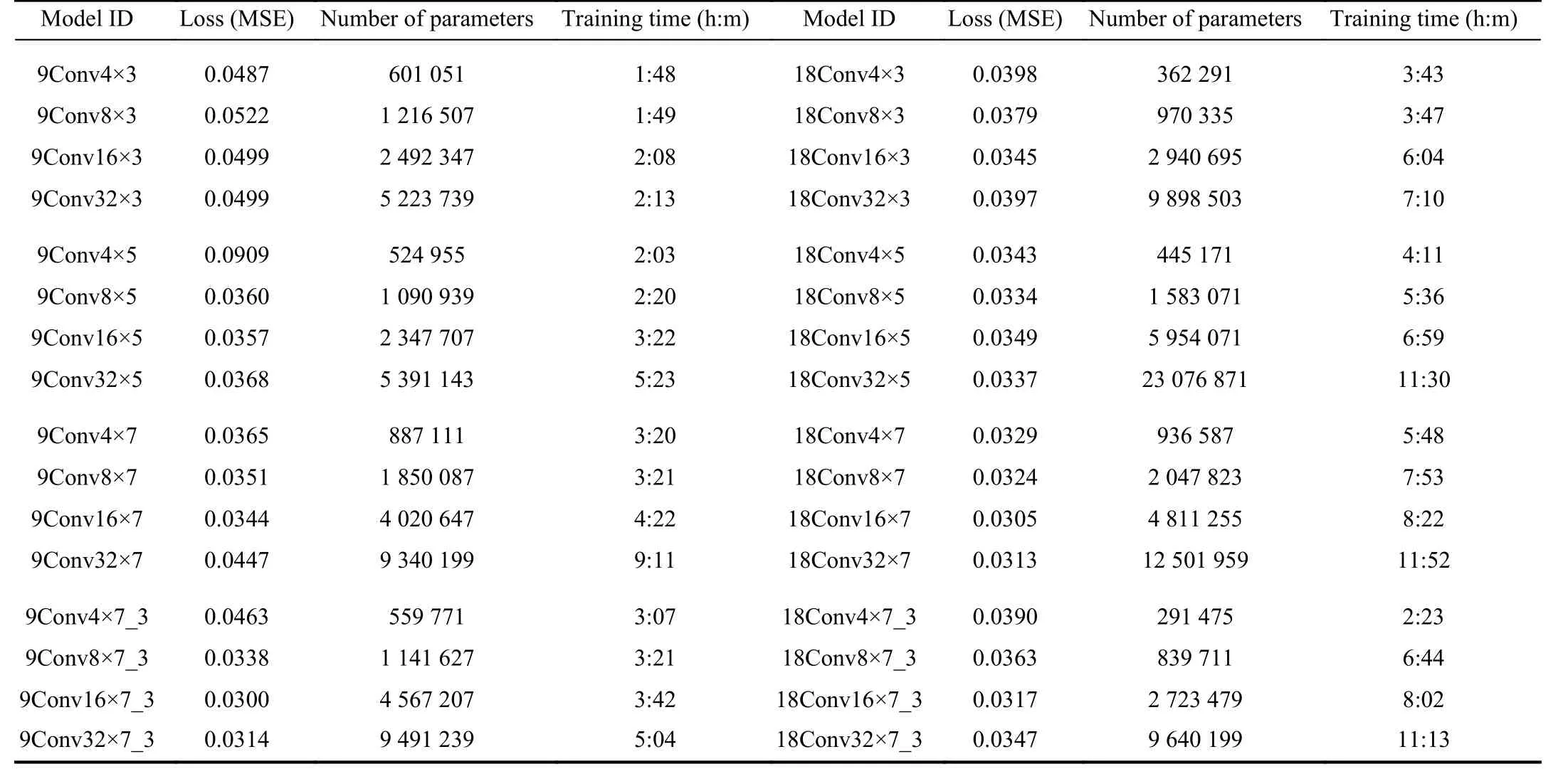
TABLE III (continued)NUMERICAL PERFORMANCE RESULTS OF THE TRAINED CNN MODELS