Estimation of leaf color variances of Cotinus coggygria based on geographic and environmental variables
Xing Tan · Jiaojiao Wu · Yun Liu · Shixia Huang · Lan Gao · Wen Zhang
Abstract Capturing leaf color variances over space is important for diagnosing plant nutrient and health status, estimating water availability as well as improving ornamental and tourism values of plants. In this study, leaf color variances of the Eurasian smoke tree, Cotinus coggygria were estimated based on geographic and climate variables in a shrub community using generalized elastic net (GELnet) and support vector machine (SVM) algorithms. Results reveal that leaf color varied over space, and the variances were the result of geography due to its effect on solar radiation, temperature, illumination and moisture of the shrub environment, whereas the influence of climate were not obvious. The SVM and GELnet algorithm models were similar estimating leaf color indices based on geographic variables, and demonstrates that both techniques have the potential to estimate leaf color variances of C. coggygria in a shrubbery with a complex geographical environment in the absence of human activity.
Keywords RGB color space · Digital elevation model · Variable selection · SVM algorithm · GELnet algorithm
Introduction
Numerous digital methods based on spectral reflectance have been applied in order to quantify leaf color of plants rapidly and accurately. Among these methods, satellite technologies can capture spectral information of plant foliage at a large scale (Li et al. 2014), but application is constrained by cost, the risk of fuzzy images caused by clouds, and the low accuracy due to background soil interference (Chen et al. 2010; Wang et al. 2014). In contrast, digital still camera imagery, with the advantages of simplicity and ease of use, low cost, and high spatial and temporal resolution, has been applied extensively to obtain the information on leaf color (Wang et al. 2014). The images produced by digital still cameras include considerable information on leaf color. This information is relatively easy to separate and extract from background and other interferences using existing image processing software (Li et al. 2010). The common color spaces of the images include RGB, HSV, and CIE L * a * b * spaces, and the color indices based on these color spaces have been widely used in the studies of plant characteristics (Wang et al. 2014; Fernandez-Gallego et al. 2019). However, the precision of images from digital still cameras is subject to light intensity (Karcher and Richardson 2003; Wang et al. 2013; Vesali et al. 2015). An effi cient method for reducing the effect of light intensity changes on image information is to use combination indictors such as dark green color index (DGCI) (Rorie et al. 2011; Wang et al. 2014; Vesali et al. 2015). Karcher and Richardson ( 2003) reported that the green indictor from RGB space cannot depict the extent of green for turf grass completely, while the dark green color index (DGCI) from HSV color space was more consistent with how the green color of plants appeared. In addition, to avoid the effect of illumination variations in nature on color images, some studies used special equipment such as artificial light to acquire all images in the laboratory. For example, Rorie et al. ( 2011) used a black felt background and a fluorescent light to acquire color images of corn leaves using a stationary camera set 58 cm above the leaves. In addition, owing that a * and b * are independent with luminance (L * ), the CIE L * a * b * color space as a device-independent color space can accurately depict the variances of leaf color without the interference of light intensity (Wang et al. 2014).
Autumn colored plants [e.g. Cotinus coggygria Scop., Ailanthus altissima (Mill.) Swingle, and Acer palmatum Thunb.] with ornamental and tourism values have attracted considerable attention (Lev-Yadun and Gould 2007; Lev-Yadun 2010). Leaf color is an important indicator of physiological status for an autumn colored plant, and can provide essential information for ecological modelling, environmental prediction, and tourism resource management (Dutta Gupta et al. 2013; Wang et al. 2014; Vesali et al. 2015; Lang et al. 2017). For example, chlorophyll and nitrogen content of leaf tissues can be estimated by color indictors because of their close correlation with and chlorophyll or nitrogen content (Vollmann et al. 2011; Vesali et al. 2015; Rigon et al. 2016).
Leaf color variations of autumn colored plants is an adaptive response to environmental variations (Prasad and Iverson 2003; Keenan et al. 2014; Xie et al. 2015, 2018). Climate is considered to be the primary control of leaf color variations (Estrella and Menzel 2006), and conditions of temperature and precipitation show significant correlation with leaf color in most autumn colored plants (Archetti et al. 2013; Keenan and Richardson 2015; Xie et al. 2018). In general, cool temperatures and heavy rains advance color changes in plants while warm temperatures and drought or low rainfall delay color changes (Estrella and Menzel 2006; Keenan and Richardson 2015). In addition, the phenological response by different plants to climate are different, for example, the variation of leaf color in maple species with low drought tolerance is delayed under the influence of drought, while changes in oak species with more drought tolerance are advanced (Xie et al. 2018). In fact, climatic patterns are not independent of the influence of geography and disturbance factors (e.g., human activity and features of biological community) (Wang et al. 2006). Since the climatic environment (e.g., solar radiation, temperature, illumination and moisture) can be affected by geography, the phenological responses of autumn colored plants to environment are also affected by geographical conditions (Garonna et al. 2015; Kobayashi et al. 2016; Rozenstein and Adamowski 2017). For example, Rozenstein and Adamowski ( 2017) indicated that there were significant correlations of leaf color with elevation and latitude; the onset of leaf color change and the duration of the peak coloration phase were sooner and shorter, respectively, with increasing elevation from 500 m at northern latitudes in southern Québec, Canada. They attributed this to temperature differences caused by geography. Xie et al. ( 2018) found the responses of different species to local variations in site conditions fluctuated considerably. Thus, the impact of climate, geography and other factors, autumn leaf colors are diverse over space, especially in a shrub area with sharply rolling terrain.
Due to the statistical causal relationship between leaf color and environmental factors, it is possible to simulate color variations of autumn colored plants based on environmental factors (Estrella and Menzel 2006; Keenan and Richardson 2015). In recent years, numerous statistical methods to estimate the variances of plant properties have been used, such as multivariable linear, LASSO, stepwise, and ridge regression analysis, elastic net, and machine learning methods (Dutta Gupta et al. 2013; Vesali et al. 2015). However, the demands of most linear regression methods for data structure are high, which limits the application in plant property estimations to some extent (Broadhursta et al. 1997). The generalized elastic net (GELnet), as an extension ofelastic net regression, is able to implement correlation variable selection, improve the robustness of the model and reduce bias in estimation (Zou and Hastie 2005; Sun 2011; Friedman 2012). Most studies have demonstrated that GELnet is promising and effi cient in estimating the dependent variable based on the data with non-constant variance structures (Friedman 2012), but its application in explaining plant properties has not been developed. Besides, machine learning methods such as support vector machine (SVM) with less demands on data structure, and with the ability to catch non-linear relationships as well as address the overfitting problem, has been extensively used in plant property assessments (Yuan et al. 2017; Gerhardt et al. 2019; Hao et al. 2019). Nevertheless, most studies have concentrated on plant features such as chlorophyll, nitrogen, leaf weight, area, edge, and defoliation using these regression methods (Dutta Gupta et al. 2013; Wang et al. 2014; Vesali et al. 2015; Yuan et al. 2017; Liang et al. 2018). The exploration and quantification of leaf color variations based on the relationships between color and environmental factors in a shrub ecosystem with complex topography has not been reported.
Many colored-leaf plants (e.g., C. coggygria, Ginkgo biloba L., A. palmatum, and Pistacia chinensis Bunge) provide economic value in addition to beautifying the environment, and have been widely used in gardens and tourist locations (Liu and Gao 2010; Zhang and Goldberg 2011). Determining the variation in leaf color over space is critical for improving ornamental and tourist values of leaf colored species. Therefore, in this study, leaf color indices of C. coggygria from color digital images were developed (1) to analyze the variances in color; (2) to reveal the relationships between leaf color and environmental factors; and, (3) to investigate the potential ofenvironmental factors for estimating leaf color variances using GELnet and SVM models.
Materials and methods
Study area
Samples of C. coggygria leaves were collected from three natural scenic areas, Huangyan, Goddess Peak and Wenfeng, which are the main distribution areas of C. coggygria within Wushan County of Chongqing, China (109°33′?110°11′ E, 23°28′?30°45′ N). The region is typical of karst landforms created by the dissolution of soluble rocks such as limestone, and with alternating deep valleys and mid-level mountains. The study area has undulating topography with elevations from 73 m to 2680 m a.s.l. It is located in a moderately subtropical zone and receives over 1570 h of sunshine annually, more than 1055 mm of precipitation, with approximately 68% relative humidity. Average temperatures are 18.2 °C with approximately 320 frost-free days yearly. With the increase in elevation, temperatures, precipitation and frost-free days at about 0.66 °C, 55 mm and 10 days for every 100 m increase in elevation. Soil types are mainly Lithic Udorthents with high calcium carbonate content and Dystrochrepts with base Saturation < 20% (Soil Survey Staff 2010).
Considering the variations in terrain of the study area, we collected ninety-six samples of C. coggygria leaves from shrub communities of Huangyan, Goddess Peak and Wenfeng scenic spots in late November 2018 when most leaves had turned red (Fig.1). To ensure the samples reflected leaf color changes as widely as possible, we collected eight healthy leaves from different parts of the shrub. Each sample, was placed in a plastic bag, sealed, placed in an insulation bucket with ice, and transported to the laboratory for digital imaging.
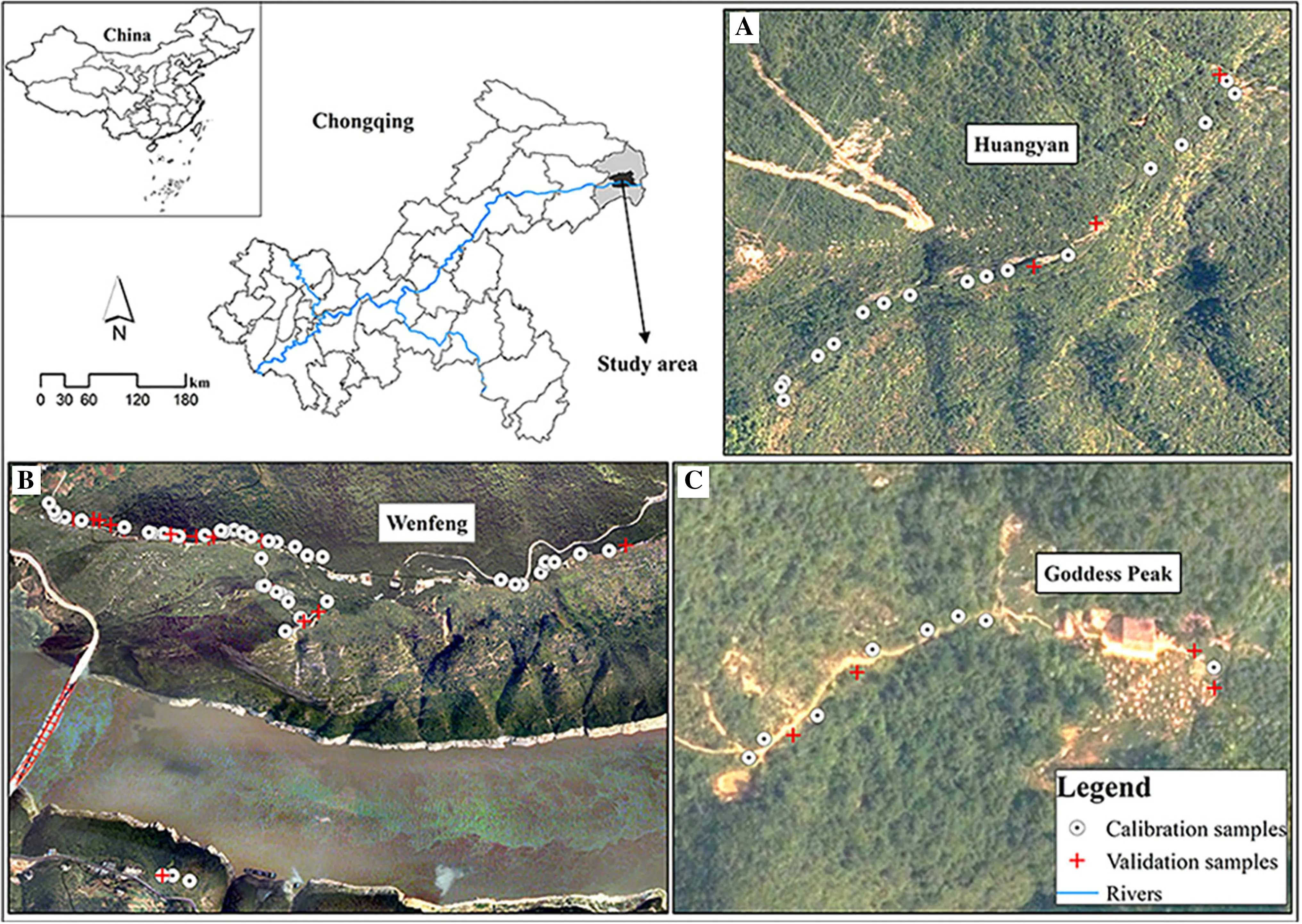
Fig.1 Distribution of samples in the study area: a Huangyan, b Wenfeng and c Goddess Peak
A Canon EOS 7D Mark II (Canon Inc., Tokyo, Japan) digital still camera positioned 50 cm above the material was used for recording digital images. The camera lens was set at an aperture of five with automatic shutter speed adjustment, focal length of 37 mm, auto white balance, auto exposure time and auto-focus with the flash off . Each leaf was washed with deionized water and placed on the laboratory table for photographing. A white A4 paper was used as background for ease of segmenting the images. All digital images were stored in JPEG (Joint Photographic Experts Group) file format with a resolution of 3648 × 2432.
Image processing and color indices extraction
Because the digital images contained leaf blade, petiole, stipule and a white background, the images need to be segmented to retain only leaf blades. Segmentation was implemented using Adobe Photoshop CS6 software (Adobe Systems Inc., CA, USA). All segmented images were stored in PNG (Portable Network Graphics) file format with lossless compression characteristics.
The RGB space is the most commonly model for mirroring color information of image, which was built based on three primary colors including red (R), green (G), and blue (B). The brightness value ofeach primary color ranges from 0 to 250. In this study, all raw images of leaves taken by camera were made up of RGB space. After the digital image segmentation, values of RGB space were extracted from the segmented digital images. The RGB values ofeach image were the mean values of all the pixels, hence the RGB values ofeach sample were the mean values of all images among a sample.
As a hexagonal cone model, HSV space is a common color space built by Smith ( 1978) based on the intuitive nature of color. The hue (H), the pure spectrum of colours with a range from 0° to 360° in HSV space, represents a monochrome of the visible spectrum; saturation (S) represents the degree of the color to the spectrum color with values between 0 and 1; and, brightness (V) refers to the brightness of the color not directly related to light intensity, the value range which is the same as that of S. The formulas for quantifying the HSV values are as follows (Vesali et al. 2015):
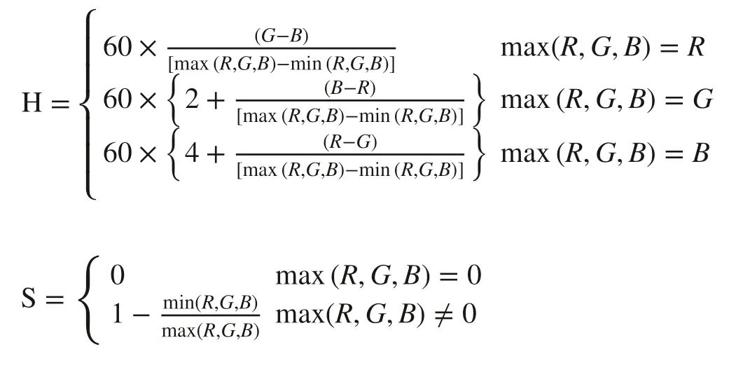

where R, G, and B are digital values for red, green, and blue channel of RGB space.
CIE L * a * b * space is a device-independent color system based on physiological characteristics which was established by the International Commission on illumination (CIE) in 1931. The L * in CIE L * a * b * space represents color luminance, while a * and b * represents red-green and yellow-blue chroma, respectively. The CIE L * a * b * space was acquired by the conversion formulas as follows (Robertson 1977; Wiwart et al. 2009):
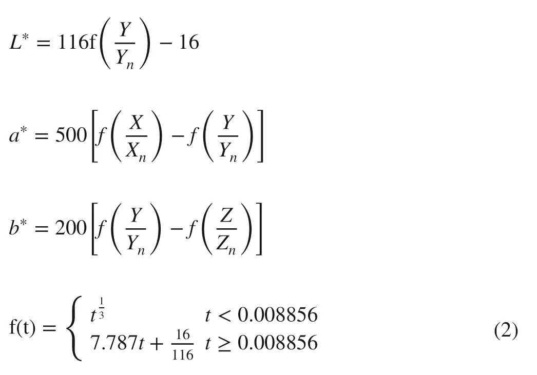
where Xn, Yn, and Znare the tristimulus values of a standard illuminator; X, Y, and Z are the tristimulus values of color converted by RGB space.
In addition, the other combination indices including intensity (INT) (Wang et al. 2014) and dark green color index (DGCI) (Vesali et al. 2015) were obtained based on RGB space and HSV space respectively as follows:

In this study, all color indices extractions were done with Matlab 7.12.0 software (MathWorks Inc., Natick, MA, USA). For HSV and CIE L * a * b * color space, the “rgb2hsv” and “srgb2lab” functions were used to calculate their values, respectively.
Geography and climate data
A digital elevation model (DEM) with 5 m spatial resolution was used. In order to improve the precision and speed of calculation, the DEM preprocessing, including clipping, and filling, was carried out. After pretreatment, the 17 geographic variables selected were (Fig.2): elevation (Ele), slope (Slope), aspect (Aspect), catchment area (CA), catchment slope (CS), diurnal anisotropic heating (DAH), flow line curvature (FLC), local upslope curvature (LUC), ls factor (LSF), maximum height (MH), melton ruggedness number (MRN), slope height (SH), surface area (SA), topographic wetness index (TWI), wind exposition (WE), latitude (Lat), longitude (Lon). DEM processing and all terrain index extractions were implemented in SAGA GIS 7.2.0 software.
Climate data, including daily minimum, maximum and mean temperatures, daily precipitation, daily mean and minimum relative humidity in 2018 from 63 weather stations, were provided by the Chongqing Meteorological Information and Technical Support Center (Fig.2). According to sampling time, these climate data from January to November in 2018 were further used to calculate average annual minimum, maximum, and mean temperatures (Tmin), (Tmax), and (Tmean), respectively, average annual precipitation (Pre), average annual and minimum relative humidities (RHmean), and (RHmin), respectively. To extract the climate indices of each sample, climatic maps of the study area were obtained using the thin-plate spline (TPS) method with climate data from 63 weather stations. Climatic variables corresponding to the sample points were extracted for further analysis. All climate data were processed in R v3.5.1 software (R Development Core Team 2018).
The results of correlation analysis between geographic and climate variables using Pearson correlation analysis is shown in Fig.3. There are significant correlations ( p < 0.05) between most environmental variables.
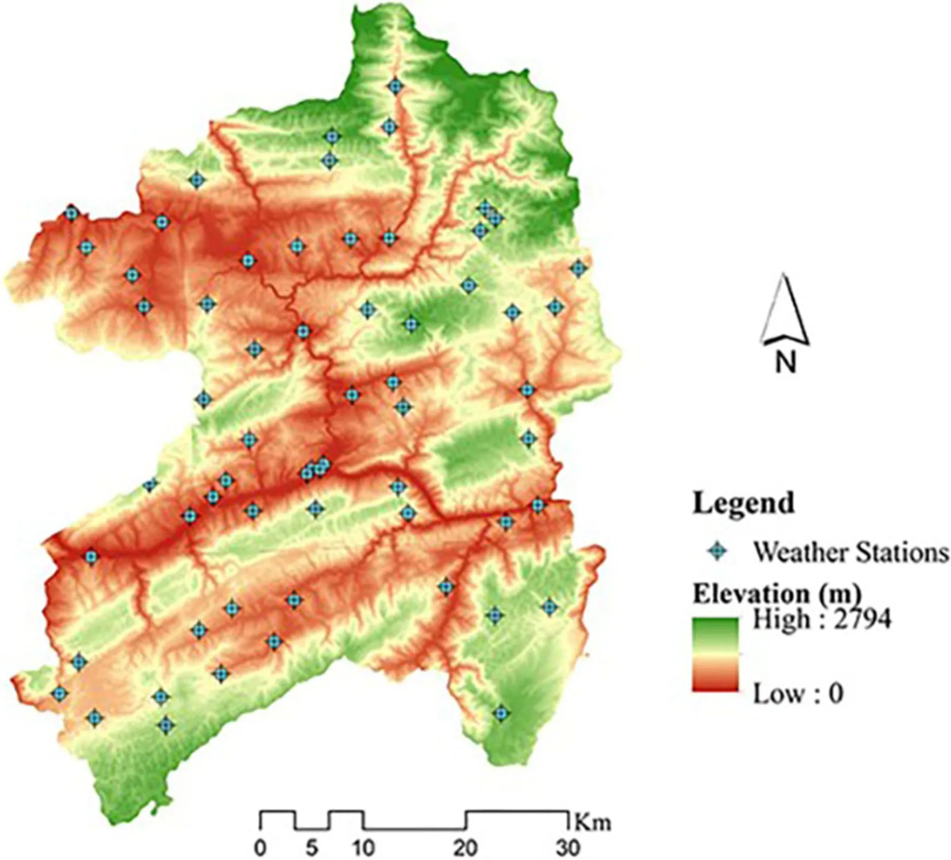
Fig.2 Distribution of weather stations and digital elevation model of the study area
Methodology
The generalized elastic net (GELnet) model is a linear regression developed from the elastic net model (Zou and Hastie 2005). Based on the nonconvex optimization problem, the GELnet model can result in more sparse solutions, improve the robustness of the model and reduce bias in estimation by controlling the model complexity and avoiding over-fitting and singularity problems (Chartrand 2007; Sun 2011; Friedman 2012). Furthermore, the GELnet model with sparseness can be used to select variables. When multiple independent variables are highly correlated, the model can make a trade-off between one and a group of independent variables. In order to reduce the influence of highly correlated variables on the regression models, in this study the GELnet method was applied to variable selection before the regression models were established. In the model, the optimal combination of variables was determined by Mallows’ Cpcriterion (Cp), which is an unbiased estimator of the true prediction error. Cpcan be defined by (Efron et al. 2004):


The Cpcan be used to determine model complexity and performance; model performance with minimum Cpis generally the best (Hirose et al. 2011). Thus, the optimal combination of variables from the optimal GELnet model, selected by the Cp, was used for further research (Fig.4). A detailed description of the GELnet model is found in Hirose et al. ( 2011), Friedman ( 2012), and Zhang et al. ( 2017).
For the GELnet model, the “msgps” package in R was used (Hirose 2019). After several experiments, most leaf color indices (except the index of a * ) could be estimated based on the corresponding optimal combination of geographic variables using the GELnet model, whereas climate variables failed to explain the variances of all leaf color indices (Table 1). To compare models, performance, the SVM and GELnet models ofeach leaf color index were established based on the same combination ofenvironmental variables (Table 1).

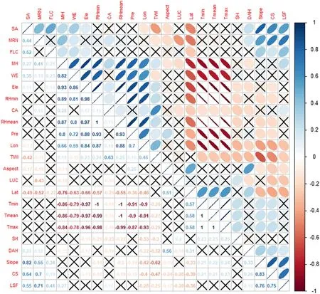
Fig.3 Correlation coeffi cients ofenvironmental variables; × denotes non-significant correlations ( p > 0.05) between environmental variables
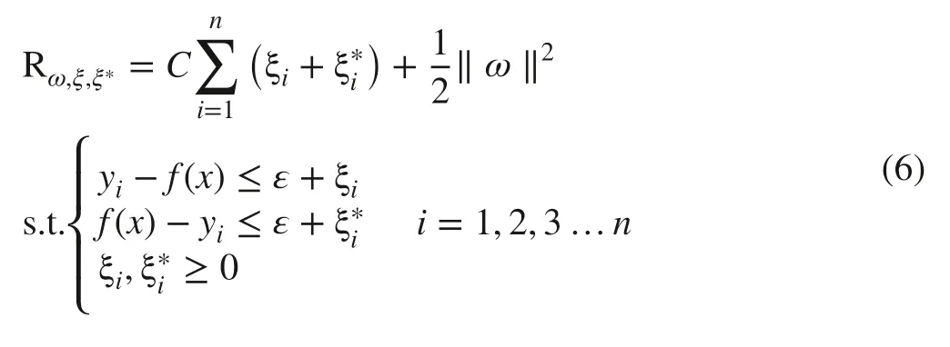
where ε is an insensitive coeffi cient, yithe output value of the i th data ( i = 1,2,3,…, n), C a penalty factor. Finally, by introducing the Lagrange function (ai, ai*), Eq. ( 6) can be converted into a dual problem for optimizing the convex quadratic programming and the expression of f(x) can be written as:

where v is the number of support vectors, aiand ai* the Lagrange factors.
Moreover, the SVM model also introduces a kernel function to solve the non-linear regression problem. In this study, four common kernel functions (linear, polynomial, radial basis, and sigmoid) were used to produce the SVM model for each color index, and then the kernel function with the highest precision in the model was selected for further analysis. After several experiments, the polynomial function as the kernel function in SVM model was selected for G, the radial basis function selected for R, S, L * and b * , and the sigmoid function for H, V, INT andDGCI. All SVM models were accomplished in R v3.5.1 software (R Development Core Team 2018) using the “e1071” package.
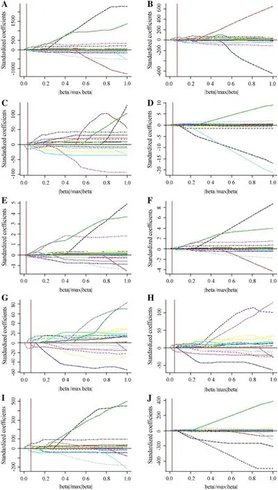
Fig.4 Solution paths of GELnet models for leaf color indices: ( a) R, ( b) G, ( c) B, ( d) H, ( e) S, ( f) V, ( g) L * , ( h) b * , ( i) INT and ( j) DGCI; vertical line denotes the selected model by the C p ; R, G, and B are digital values for red, green, and blue channel of RGB space; H, S, and V are digital values for hue, saturation, and brightness channel of HSV space; L * and b * are digital values for luminance, red-green and yellow-blue channel of CIE L*a*b* space; INT and DGCI denote intensity and dark green color index, respectively
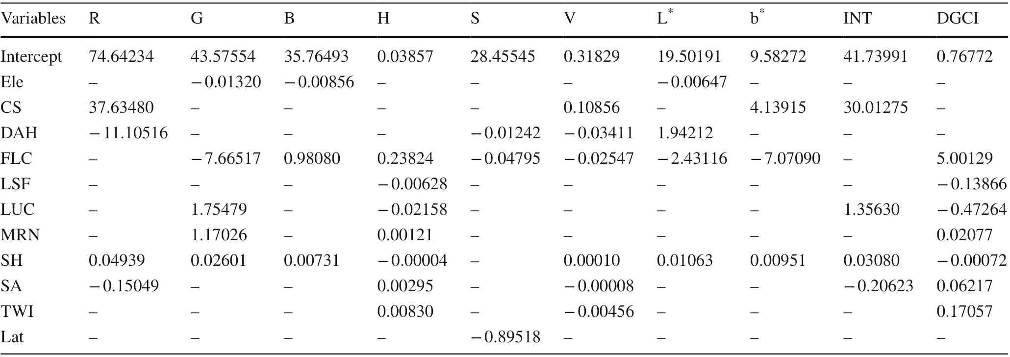
Table 1 Coeffi cients of geographic variables in optimal GELnet model for estimating leaf color indices
Descriptive statistical analysis was applied to test the variances of leaf color indices, Spearman’s correlation coeffi cient used to explore the relationships between leaf color indices and environmental variables, and the one-way analysis of variance (ANOVA) with least-significant difference (1.s.d.) test used to determine the differences in leaf color indices at different elevations. All statistical analyses were calculated in SPSS 19.0 software (IBM Co., Chicago, MI, USA).
Validation
An independent dataset (24 samples) as a validation set, randomly selected from the 96 sample dataset, was used to determine model performance. Accuracy indicators, including mean absolute error ( MAE), relative root mean squared error ( RRMSE), Lin’s concordance correlation coeffi cient ( LCCC), and the coeffi cient of determination ( R 2 ), were calculated by the observed and predicted values based on the validation set. The expression of these accuracy indicators is defined as:

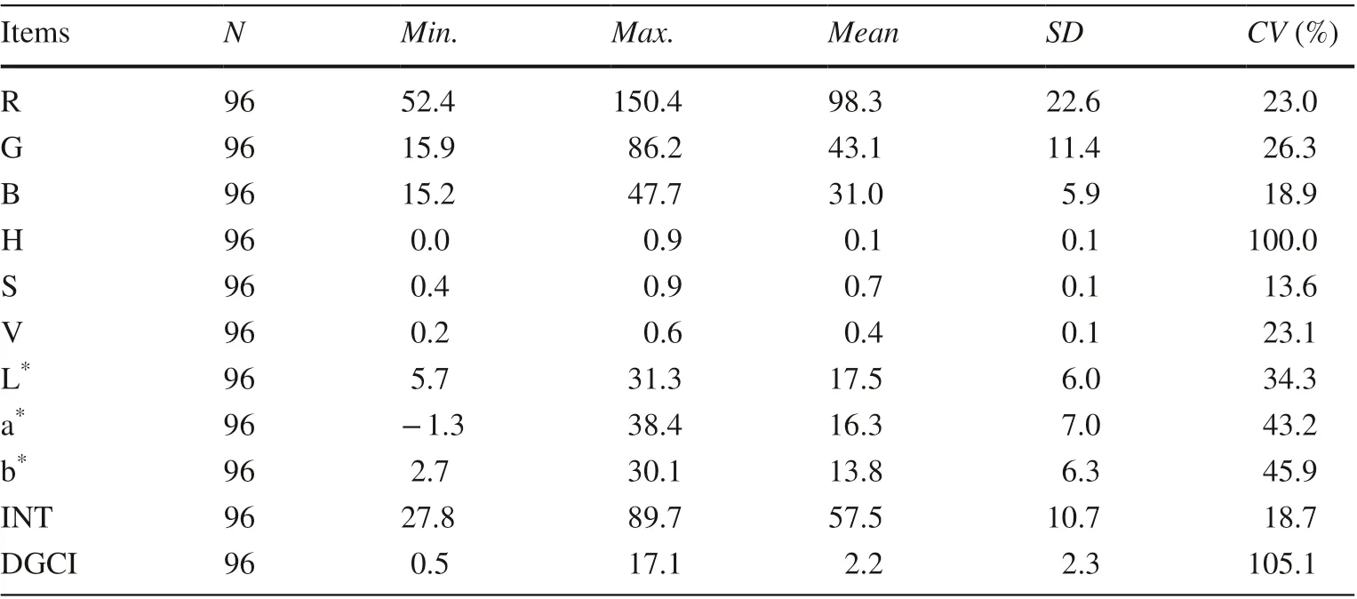
Table 2 Descriptive statistical analysis of leaf color index
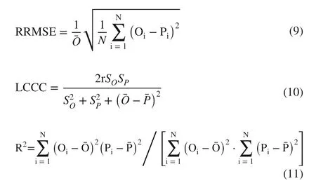
where r and N are the correlation coeffi cient and the number of validation datasets respectively; Oiand Piare the observed and predicted values, respectively;andare the mean values ofobserved and predicted values, respectively;andare the standard deviations ofobserved and predicted values, respectively. Models with lower MAE, RRMSE and higher LCCC , R 2 performed better.
Results
Descriptive analysis of leaf color
Except for the dark-green colour index (DGCI), the coefficients of variation ( CV) for all leaf color indices were between 10 and 100%, which indicates that leaf color index had intermediate variation, while the DGCI with a CV (105.12%) of more than 100% represented strong variability (Table 2 ).
Correlation between leaf color indices and environmental factors
Ele (elevation) had negative correlation with most color indices (except H, S and DGCI), and correlation with G ( r = ?0.247, p < 0.05), B ( r = ?0.326, p < 0.01), H ( r = 0.211, p < 0.05), DGCI ( r = 0.207, p < 0.05), and L * ( r = ?0.293, p < 0.01) reached significant levels. MH (maximum height) was significantly negatively correlated ( p < 0.05) to B and L * , but positively correlated ( p < 0.05) to H (hue) and DGCI. SH (slope height) was positively correlated with R, G, B and INT (intensity). In addition, significant negative or positive correlations ( p < 0.05 or 0.01) existed between other geographic variables (catchment area, CA; catchment slope, CS; diurnal anisotropic heating, DAH; local upslope curvature, LUC; topographic wetness index, TWI; wind exposition, WE; longitude, Lon; and latitude, Lat) and leaf color indices (Table 3).
Correlation coeffi cients between color indices and climate variables were lower (Fig.5). Only the correlation of climatevariables for G, B and L * were significant ( p < 0.05 or 0.01), indicating that climate had an impact on leaf color, but the interpretation of climate variables for most of color indices were lower.

Table 3 Correlation coeffi cients between leaf color indices and geographic variables
Estimation of leaf color index based on GELnet and SVM models
For all color indices, the R 2 values in the GELnet and SVM models ranged from 0.134 and 0.153, to 0.467 and 0.339, respectively (Fig.6). All environmental variables were not selected in GELnet model for explaining the variance of a * , hence data on leaf color index a * are not shown in further analysis.
By comparing accuracy indicators, SVM models gave slightly lower MAE, RRMSE, and higher LCCC, R 2 than that of the corresponding GELnet models on the prediction of most color indices (Table 4). However, the differences in performance were not obvious between the models.
Discussion
As a typical karst landform, the study area had been gradually created by the destruction of the original vegetation (broad-leaf forest) through anthropogenic activities and, consequently, serious soil erosion in the 1960s and 1970s. The shrub community, consisting largely of C. coggygria, did not appear until the 1980s. Over the sharply rolling terrain and vegetation succession processes, the distribution of the shrub community is discontinuous. Therefore, this study focused only on the location of a shrub community with less human disturbance.
The SVM model was slightly superior to the GELnet model in comparing accuracy indicators, possibly benefitting from generalization, avoiding overfitting, and local minimum problem (Ben-Hur and Weston 2010) (Table 4). However, there was little difference in performance between the two models. The GELnet model improved robustness, reduced estimation bias, and estimated leaf color indices effectively. Additionally, the GELnet model, as an extension ofelastic net bridging the lasso and ridge-regressions, had advantages over the SVM model such as its simplicity, ease of use, straightforward interpretation, and the ability to deal with the problem of collinearity (Friedman 2012). There were highly correlations between environmental variables (Fig.3), which could lead to a collinearity problem in prediction models. In order to reduce this effect, the GELnet model was implemented to obtain optimal combinations of variables for leaf color indices before building the prediction models. The variance inflation factor ( VIF) of the variables for all color indices were less than 10 (Supplementary File Table 1), which suggests that there were no collinearity problem in the models (Alauddin and Nghiemb 2010).
Climate is an importance factor in affecting the leaf color variances, and most previous research has indicatedthat color varies remarkably with changes in climate during the complete cycle of leaf color variances (Archetti et al. 2013; Keenan and Richardson 2015; Xie et al. 2018). However, in this study, correlation analysis and variable selection results suggest that the effects of climate variables on leaf color of C. coggygria seem to be discounted, which is not in agreement with the results of previous research (Archetti et al. 2013; Xie et al. 2018). This could be related to time of sampling which, in this study, was carried out in late November when most leaves had changed color and climate was relatively consistent over space, with CV < 10% for all climate variables (Fig.7). As a result, variances ofcolor over the area was controlled mainly by topography, but not by climate. Rozenstein and Adamowski ( 2017) found that greater inter-annual variation of autumn foliage color resulted from climate variations in southern Québec, Canada during 2011–2015. In this study area with complex topography, however, it is highly uncertain whether climate is closely correlation with leaf color variation over space at an inter-annual scale. Therefore, a longer time period is required to further explore the relationships
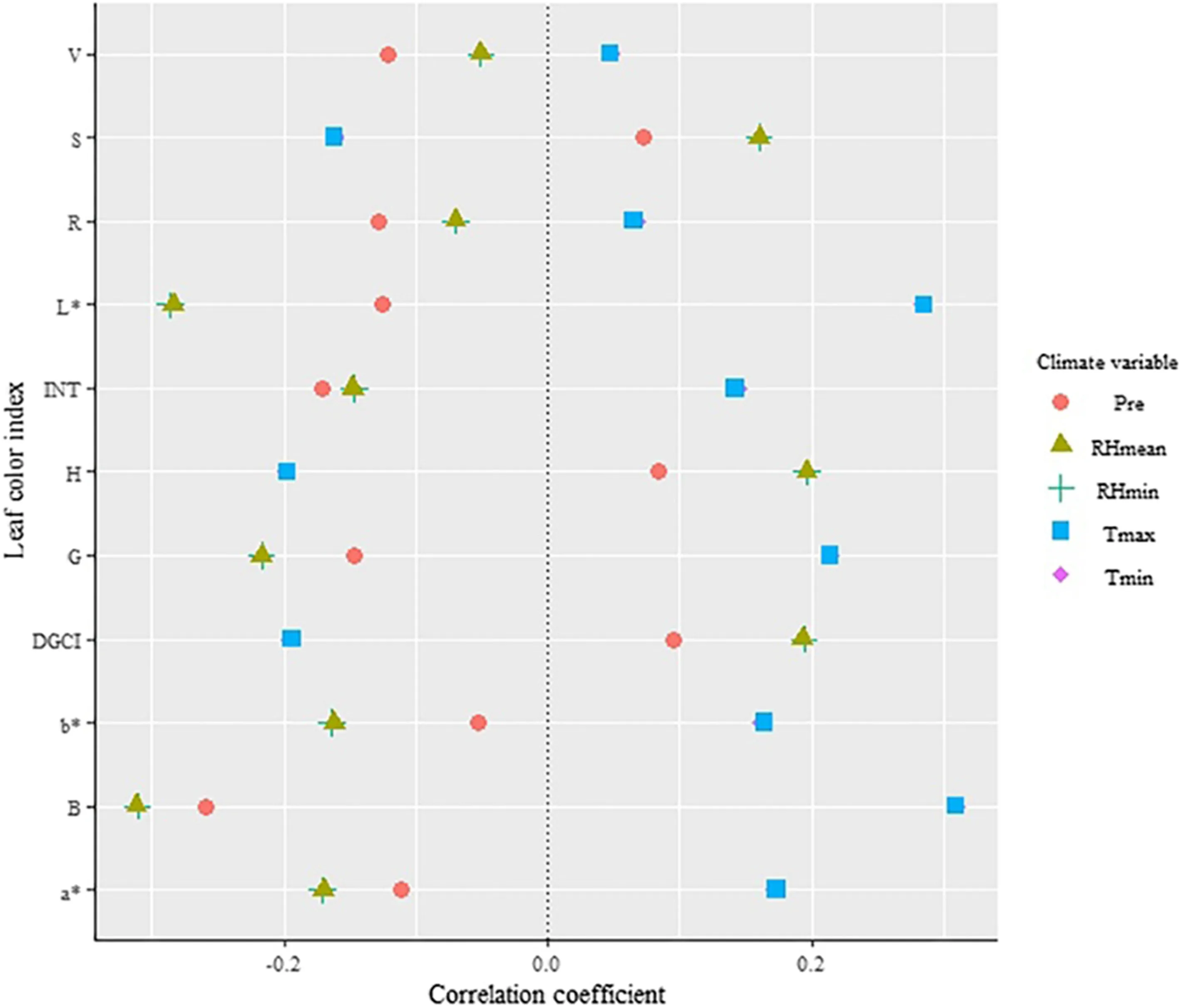
Fig.5 Correlation coeffi cients of leaf color indices with climate variables
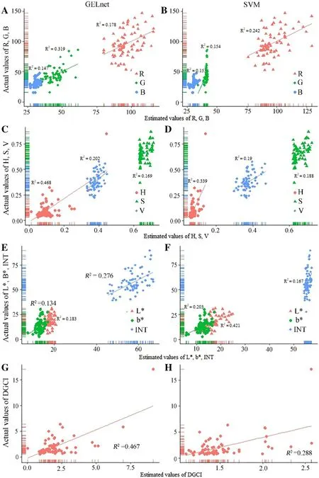
Fig.6 Comparisons of GELnet and SVM models from calibration dataset for leaf color indices: ( a) R, G, B, ( b) H, S, V, ( c) L * , b * , INT, and ( d) DGCI
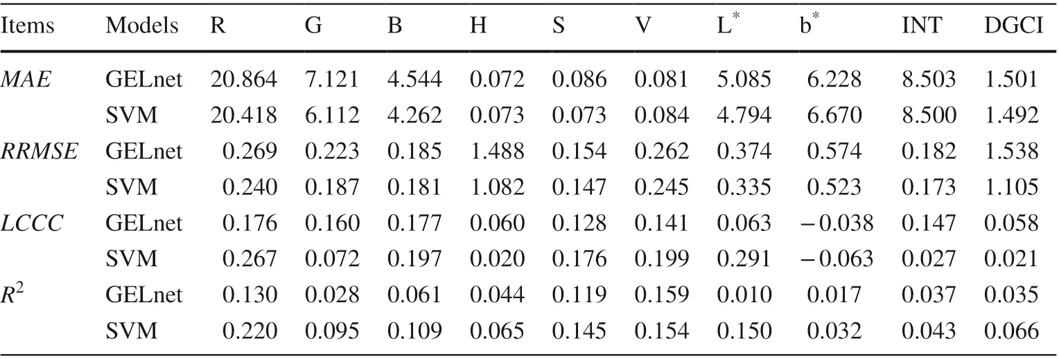
Table 4 Performance of GELnet and SVM models for estimating leaf color indices with geographic variables
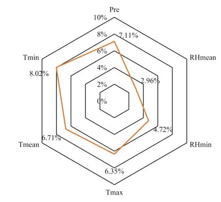
Fig.7 Coeffi cients of variation ( CV) of climate variables
Topography indirectly controls variances in leaf color by affecting solar radiation, temperature, illumination and moisture, especially in a shrub community on sharply rolling terrain (Rozenstein and Adamowski 2017). This study verified the important of topography in affecting the variances of leaf color by correlation analysis and regression models. In general, leaves may be much redder at higher altitudes due to the increase in anthocyanins, responsible for red coloration, and the degradation of chlorophyll with decreasing temperatures (Kobayashi et al. 2016; Rozenstein and Adamowski 2017). Moreover, there are significant differences in the color of leaves in regions at the same attitudes influenced by complextopography. However, this study indicated that most of leaf color indices at different elevations were not significantly different ( p > 0.5), while medium or strong variability of leaf color indices at the same elevation still exists ( CV > 10%) (Table 5). In addition, the coeffi cients of independent variables in the GELnet model show that elevation was the not most important factor for explaining variances in leaf color indices, and not even selected in some models. A possible explanation for this might be the stability and heterogeneity of the anthocyanin content in C. coggygria leaves. Over the sampling period (late November), most leaves turned red. Anthocyanin contents of most leaves tended to be stable and the differences of leaf color decreased at different altitudes. In regions with similar attitudes, the effect ofelevation on leaf color tends to be constant, and temperature, illumination and moisture are not invariant over space under the influence ofother terrain variables (e.g. flow line curvature, slope height, and topographic wetness index). Anthocyanin contents of leaves were heterogeneous over space in specific environments which led to significant variability in coloration of C. coggygria leaves.

Table 5 Coeffi cients of variation ( CV) and differences of leaf color indices for different elevations
It is important to note that, while some variances of color indices could be estimated by the SVM and GELnet models, most remained unexplained. This might be related to some over-looked factors, such as soil properties, which were verified to be important in affecting leaf color (Prasad and Iverson 2003). Climate has a remarkable influence on leaf color but the impact was reduced by the time of sampling in this study. Keenan and Richardson ( 2015) noted that autumn phenology of plants is correlated with spring, and the response in autumn to climate is influenced by seasonal spring changes. Thus, spring growth phenomena as related to climate should be studied to explore phenological changes (e.g., leaf color, leaf drop) in the following autumn (Xie et al. 2018). Sample size is a critical factor in estimating variances of leaf color indices. The performance of the model is closely related to sample size, and performance with a large sample is generally better. In this study, only 96 samples were used to produce the model for estimating variance of leaf color indices. The sample size was too small to capture completely, by prediction models, the relationships between leaf color indices and environmental variables as well as the variance patterns of leaf color indices. Long-term phenology observations with a lager sample size and more factors (e.g., soil properties) should be considered for future research to improve model performance and reveal more accurately patterns of leaf color variance over space.
Conclusion
An interesting finding of this study was that geography was significantly correlated with leaf color variances, attributed to its effect on solar radiation, temperature, illumination and moisture, whereas the direct influences of climate were not obvious. The SVM and GELnet models were similar in estimating leaf color indices based on geographic variables, which suggests that both models may serve as useful tools for estimating the leaf color variances. However, subject to sample size and other factors, the ability to explain SVM and GELnet models to leaf color variances of C. coggygria were not perfect.
AcknowledgementsWe thank the Chongqing Meteorological Information and Technical Support Center for providing climate data.
References
Alauddin M, Nghiemb HS (2010) Do instructional attributes pose multicollinearity problems? An empirical exploration. Econ Anal Policy 40(3):351–361
Archetti M, Richardson AD, O’Keefe J, Delpierre N (2013) Predicting climate change impacts on the amount and duration of autumn colors in a New England forest. PLoS ONE 8(3):e57373
Ben-Hur A, Weston J (2010) A user’s guide to support vector machines. Methods Mol Biol 609:223–239
Broadhursta D, Goodacre R, Jones A, Rowland JJ, Kell DB (1997) Genetic algorithms as a method for variable selection in multiple linear regression and partial least squares regression, with applications to pyrolysis mass spectrometry. Anal Chim Acta 348:71–86
Chartrand R (2007) Exact reconstruction of sparse signals via nonconvex minimization. IEEE Signal Process Lett 14(10):707–710
Chen PF, Haboudane D, Tremblay N, Wang JH, Vigneault P, Li BG (2010) New spectral indicator assessing the effi ciency of crop nitrogen treatment in corn and wheat. Remote Sens Environ 114(9):1987–1997
Cortes C, Vapnik V (1995) Support-vector networks. Mach Learn 20(3):273–297
Dutta Gupta S, Ibaraki Y, Pattanayak AK (2013) Development of a digital image analysis method for real-time estimation of chlorophyll content in micropropagated potato plants. Plant Biotechnol Rep 7(1):91–97
Efron B, Hastie T, Johnstone I, Tibshirani R (2004) Least angle regression. Ann Stat 32(2):407–451
Estrella N, Menzel A (2006) Responses of leaf colouring in four deciduous tree species to climate and weather in Germany. Climate Res 32:253–267
Fernandez-Gallego JA, Kefauver SC, Vatter T, Aparicio Gutiérrez N, Nieto-Taladriz MT, Araus JL (2019) Low-cost assessment of grain yield in durum wheat using RGB images. Eur J Agron 105:146–156
Friedman JH (2012) Fast sparse regression and classification. Int J Forecast 28:722–738
Garonna I, Jong R, Wit AJW, Mücher CA, Schmid B, Schaepman ME (2015) Strong contribution of autumn phenology to changes in satellite-derived growing season length estimates across Europe (1982–2011). Glob Change Biol 20(11):3457–3470
Gerhardt N, Schwolow S, Rohn S, Pérez-Cacho PR, Galán-Soldevilla H, Arce L, Weller P (2019) Quality assessment ofolive oils based on temperature-ramped HS-GC-IMS and sensory evaluation: comparison of different processing approaches by LDA, kNN, and SVM. Food Chem 286(15):307–308
Hao Z, Zhao HL, Zhang C, Wang H, Jiang YZ, Yi ZY (2019) Estimating winter wheat area based on an SVM and the variable fuzzy set method. Remote Sens Lett 10(4):343–352
Hirose K (2019) msgps: Degrees of Freedom of Elastic Net, Adaptive Lasso and Generalized Elastic Net. R package version 1.3.1
Hirose K, Tateishi S, Konishi S (2011) Effi cient algorithm to select tuning parameters in sparse regression modeling with regularization. https://arxiv.org/pdf/1109.2411.pdf. Accessed 6 Apr 2020
Karcher DE, Richardson MD (2003) Quantifying turfgrass color using digital image analysis. Crop Sci 43:943–951
Keenan TF, Richardson AD (2015) The timing of autumn senescence is affected by the timing of spring phenology: implications for predictive models. Glob Change Biol 21(7):2634–2641
Keenan T, Gray J, Friedl M, Toomey M, Bohrer G, Hollinger D, Munger JW, Okeefe J, Schmid H, Wing I, Yang B, Richardson A (2014) Net carbon uptake has increased through warminginduced changes in temperate forest phenology. Nat Clim Change 4(7):598–604
Kobayashi H, Yunus AP, Nagai S, Sugiura K, Kim Y, Van Dam B, Nagano H, Zona D, Harazono Y, Bret-Harte MS, Ichii K, Ikawa H, Iwata H, Oechel WC, Ueyama M, Suzuki R (2016) Latitudinal gradient of spruce forest understory and tundra phenology in Alaska as observed from satellite and ground-based data. Remote Sens Environ 177:160–170
Lang M, Nilson T, Kuusk A, Pisek J, Korhonen L, Uri V (2017) Digital photography for tracking the phenology of an evergreen conifer stand. Agric For Meteorol 246:15–21
Lev-Yadun S (2010) The shared and separate roles of aposematic (warning) coloration and the co-evolution hypothesis in defending autumn leaves. Plant Signal Behav 5(8):937–939
Lev-Yadun S, Gould KS (2007) What do red and yellow autumn leaves signal? Bot Rev 73(4):279–289
Li Y, Chen D, Walker CN, Angus JF (2010) Estimating the nitrogen status of crops using a digital camera. Field Crops Res 118(3):221–227
Li F, Mistele B, Hu YC, Chen XP, Schmidhalter U (2014) Reflectance estimation of canopy nitrogen content in winter wheat using optimised hyperspectral spectral indices and partial least squares regression. Eur J Agron 52:198–209
Liang WZ, Kirk KR, Greene JK (2018) Estimation of soybean leaf area, edge, and defoliation using color image analysis. Comput Electron Agric 150:41–51
Liu M, Gao CG (2010) Investigation and analysis of plant landscape during autumn and winter in Kunming city. J Landsc Res 2(10):22–26
Prasad AM, Iverson LR (2003) Little’s range and FIA importance value database for 135 Eastern US tree species. Northeastern Research Station, USDA Forest Service, Delaware
R Development Core Team (2018) R: a language and environment for statistical computing. R Foundation for Statistical Computing, Vienna
Rigon JPG, Capuani S, Fernandes DM, Guimar?es TM (2016) A novel method for the estimation of soybean chlorophyll content using a smartphone and image analysis. Photosynthetica 54(4):559–566
Robertson AR (1977) The CIE 1976 color-difference formula. Color Res Appl 2(1):7–11
Rorie RL, Purcell LC, Karcher DE, Andy King C (2011) The assessment of leaf nitrogen in corn from digital images. Crop Sci 51(5):2174
Rozenstein O, Adamowski J (2017) Linking spaceborne and ground observations of autumn foliage senescence in Southern Québec, Canada. Remote Sens 9(6):630
Smith AR (1978) Color gamut transform pairs. In: SIGGRAPH 78 conference proceedings, vol 12(3), pp 12?19
Soil Survey Staff (2010) Keys to soil taxonomy, 11th edn. USDANatural Resources Conservation Service, Washington
Sun QY (2011) Sparse approximation property and stable recovery of sparse signals from noisy measurements. IEEE Trans Signal Process 59(10):5086–5090
Vapnik V (1998) Statistical learning theory. Adaptive and learning systems for signal processing, communications, and control. Wiley, New York
Vesali F, Omid M, Kaleita A, Mobli H (2015) Development of an android app to estimate chlorophyll content of corn leaves based on contact imaging. Comput Electron Agric 116:211–220
Vollmann J, Walter H, Sato T, Schweiger P (2011) Digital image analysis and chlorophyll metering for phenotyping the effects of nodulation in soybean. Comput Electron Agric 75(1):190–195
Wang XP, Fang JY, Tang ZY, Zhu B (2006) Climatic control of primary forest structure and DBH–height allometry in Northeast China. For Ecol Manag 234(1–3):264–274
Wang Y, Wang DJ, Zhang G, Wang J (2013) Estimating nitrogen status of rice using the image segmentation of G-R thresholding method. Field Crops Res 149:33–39
Wang Y, Wang DJ, Shi PH, Omasa K (2014) Estimating rice chlorophyll and leaf nitrogen concentration with a digital still color camera under natural light. Plant Methods 10:36
Wiwart M, Fordoński G, ?uk-Go?aszewska K, Suchowilska E (2009) Early diagnostics of macronutrient deficiencies in three legume species by color image analysis. Comput Electron Agric 65(1):125–132
Xie YY, Wang XJ, Silander JA (2015) Deciduous forest responses to temperature, precipitation, and drought imply complex climate change impacts. Proc Natl Acad Sci USA 112(44):13585–13590
Xie YY, Wang XJ, Wilson AM, Silander JA (2018) Predicting autumn phenology: how deciduous tree species respond to weather stressors. Agric For Meteorol 250–251:127–137
Yuan HH, Yang GJ, Li CC, Wang YJ, Liu JG, Yu HY, Feng HK, Xu B, Zhao XQ, Yang X (2017) Retrieving soybean leaf area index from unmanned aerial vehicle hyperspectral remote sensing: analysis of RF, ANN, and SVM regression models. Remote Sens 9(4):309
Zhang XY, Goldberg MD (2011) Monitoring fall foliage coloration dynamics using time-series satellite data. Remote Sens Environ 115(2):382–391
Zhang Y, Ye WZ, Zhang JJ (2017) A generalized elastic net regularization with smoothed ?q penalty for sparse vector recovery. Comput Optim Appl 68(2):437–454
Zou H, Hastie T (2005) Regularization and variable selection via the elastic net. J R Stat Soc 67(5):768–768
 Journal of Forestry Research2021年2期
- Journal of Forestry Research的其它文章
- Stem taper functions for Betula platyphylla in the Daxing’an Mountains, northeast China
- Leaf phenotypic variation of endangered plant Tetracentron sinense Oliv. and influence of geographical and climatic factors
- Ecological variations of woody species along an altitudinal gradient in the Qinling Mountains of Central China: area-based versus mass-based expression of leaf traits
- Variations in stem radii of Larix principis-rupprechtii to environmental factors at two slope locations in the Liupan Mountains, northwest China
- A review of ecological mechanisms for management practices of protective forests
- Variation of basic density, calorific value and volumetric shrinkage within tree height and tree age of Ugandan grown Eucalyptus grandis wood
