Zhifeng ZHU(朱志鋒)

School of Mathematics and Statistics,Hubei Engineering University,Xiaogan 432000,China Hubei Province Key Laboratory of Systems Science in Metallurgical Process(Wuhan University of Science and Technology),Wuhan 430081,China

E-mail:376574200@qq.com

Shaoyi ZHANG(張紹義)Fanji TIAN(田范基)?

Hubei Key Laboratory of Applied Mathematics,School of Mathematics and Statistics,Hubei University,Wuhan 430062,China

E-mail:zhshaoyi@aliyun.com;tianfj1837@sina.com

Abstract We investigate the convergence of nonhomogeneous Markov chains in general state space by using the f norm and the coupling method,and thus,a sufficient condition for the convergence of nonhomogeneous Markov chains in general state space is obtained.

Key words f norm;coupling;nonhomogeneous Markov chains;convergence

1 Introduction

Because of the requirement of the application of Markov chains in the Monte Carlo method(MCMC),the ergodicity of time-homogeneous Markov chains has attracted considerable interest in the statistical community.The convergence of Markov chains was introduced in Meyn and Tweedie[1],Kartashov[2],Mukhamedov[3],Mukhamedov[4].Currently there already exist mature results on the convergence of the time-homogeneous Markov process in which Probabilistic Distance has been widely employed;see,for example,Theorem 5.22 and Theorem 5.23 of Chen[5].However,the ergodicity of time-homogeneous Markov chains is not enough in the application of MCMC.Therefore,it is necessary to discuss convergence of nonhomogeneous Markov chains.

Since non-homogeneous Markov chains are an extremely difficult aspect in the study of Markov processes,judging the convergence of Markov chains has been the pursuit of many scholars.The Dobrushin-Isaacson-Madsen theorem studies Markov chains in terms of finite state space(Gong and Qian[6]).In this paper,a conclusion about the convergence of nonhomogeneous Markov chains is drawn for general state space.Theorem 1.1(Dobrushin-Isaacson-Madsen theorem)is a special case of Theorem 1.2.The following Dobrushin-Isaacson-Madsen theorem gives a sufficient condition for the convergence of nonhomogeneous Markov chains in finite state space.

De finition

Let v be the signed measure on

B

(X),and let g and f be measurable functions on

B

(X).De fine

and

De finition

The Markovprocess{Φ,t∈R}is called ergodic if there is a unique invariant measure π that satis fies

De finition

Let f be measurable function on

B

(X).The Markov process{Φ,t∈R}is called f-ergodic if f≥1 satis fies that

(i) Φis a positive Harris recurrent and has an invariant measure π;

(ii) π(f)<∞;

(iii)for any initial state of x,

If f≡1,the f norm becomes the total variation norm,and accordingly,the f-ergodic becomes ergodic.

Theorem 1.1

(Dobrushin-Isaacson-Madsen Theorem[6]) Let X={X,X,···,X,···}be a non-homogeneous Markov chain in the finite state space S,and let Pbe the transfer probability matrix of its n-th step.Assume that

(A.1)there is a stationary distribution πwhen Pis a homogeneous transfer matrix;

(A.3)these either satisfy the Isaacson-Madsen condition,that for any probability distribution vectorμ,ν on S and with positive integer j,we always get

or they satisfy the Dobrushin condition,that for any integer j,if we let P=(P···P)=(P),C(P),i.e.,the contraction coefficient of P,we have

where

Then,there is a probability measure π on S such that

(1)‖π?π‖→0,n→∞;

(2)for any arbitrary initial distributionμ,the distributionμof the nonhomogeneous Markov chains always has a limit

where‖v‖is the total variation norm of the signed measure v on S.

We extend Theorem 1.1 from the finite state space S to the generalPolish space(X,ρ,

B

(X)).Let(X,

B

(X))be a Polish space,where

B

(X)is an σ algebra generated by a countable subset of X.Throughout the paper,we denote by g a measurable function on X.by v the signed measure on

B

(X),and by K a measurable nuclear on(X,

B

(X)).We de fine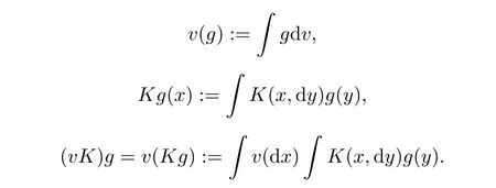

De finition

Let v be the signed measure on

B

(X),and let g and f be measurable functions on

B

(X).De fine

and

Let ?(x,y):=d(x,y)[f(x)+f(y)],where

Let Φ={Φ,Φ,···,Φ,···}be a nonhomogeneous Markov chain in(X,ρ,

B

(X)),where the transfer probability of its n-th step can be written as P(Φ∈A|Φ=x}:=P(x,A).Furthermore,if P=P=···=P,then we call Φ a time-homogeneous Markov chain.Moreover,let us de fine

P

(X)as the all probability measures on X,and xas any given point on X,and also set

M

={μ∈

P

(X):R?(x,x)μ(dx)<∞}.

Theorem 1.1 introduces the convergence of nonhomogeneous Markov chains in the finite state space.In practice,however,this is not enough.Zhang[7]introduced the existence of Markov chains coupling.Zhu and Zhang[8]studied the convergenceof nonhomogeneous Markov chains in general state space using Probabilistic Distance and the coupling method.Now,we will study the convergence of nonhomogeneous Markov chains in general state space using the f norm and the coupling method.

Theorem 1.2

Let(X,

B

(X))be a Polish space,and let Φ={Φ,Φ,···,Φ,···}be a nonhomogeneous Markov chain on X.Furthermore,let{P;n=1,2,···}be the corresponding sequence of probability kernel of Φ.Assume that

Then,there exists a probability measure π in

M

such that,for a probability measureμin

M

,we have

Remark 1

In general,the condition in the theorem(iv)is easily veri fiable.In particular,this condition is automatically satis fied when ? is a bounded distance.

Remark 2

When f≡1,the f norm becomes the total variation norm,in which case Theorem 1.2 is considered,like Theorem 1.1,a general state.

2 Preliminaries

We denote by K(μ,μ)all coupling ofμandμ.

De finition

Lettingμandμbe probability measures in the Polish space(X,ρ,

B

(X)),

Lemma 2.1

(Lindvall[9]) Letμandμbe probability measures on

B

(X),and let

Then,we have the following:

1.0 ≤γ≤1;

2.vand vare two probability measures on

B

(X);3.Q is a probability measure on

B

(X)×

B

(X).

Furthermore,let

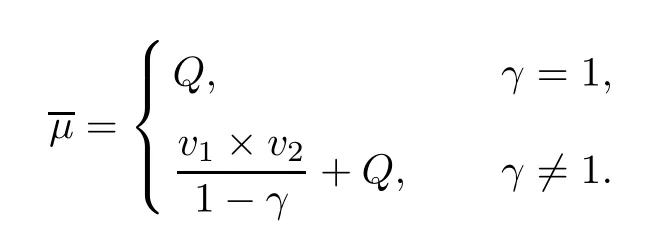
Lemma 2.2

Letμ,μbe probability measures.Hence,we obtain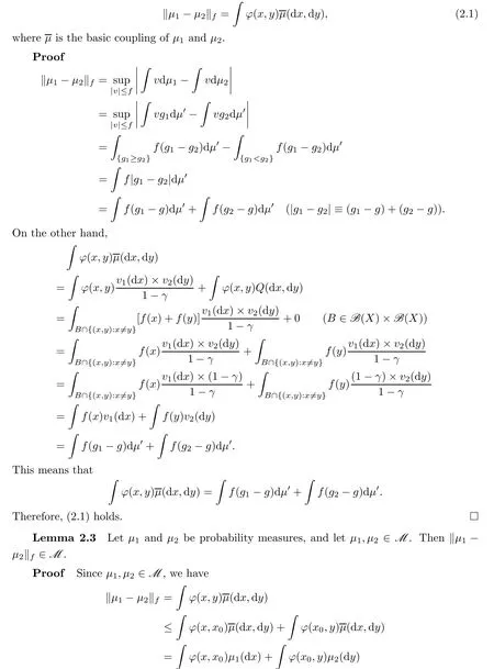

Therefore,‖μ?μ‖∈

M

.

Lemma 2.4

Letμ,μbe probability measures,and let Pbe a probability kernel on Polish space(X,ρ,

B

(X)).Assume that

Proof

From(2.2),we obtain that

As the years passed, other occasions--birthdays, recitals13, awards, graduations--were marked with Dad s flowers. My emotions continued to seesaw14 between pleasure and embarrassment.

which means that

Now we only need to prove that

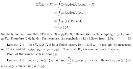
Therefore{μ:n≥1}is a Cauchy sequence.

3 Proof of the Main Result

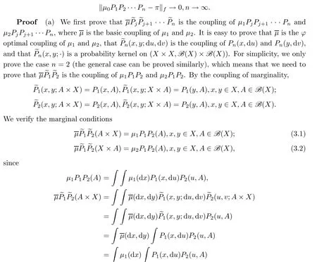
Next,we use three steps to prove The theorem 1.2:

(a)For?μ,μ∈

M

and any positive integer j,we have

(b)There exists a probability measure π∈

M

such that

Lemma 2.7 implies that{

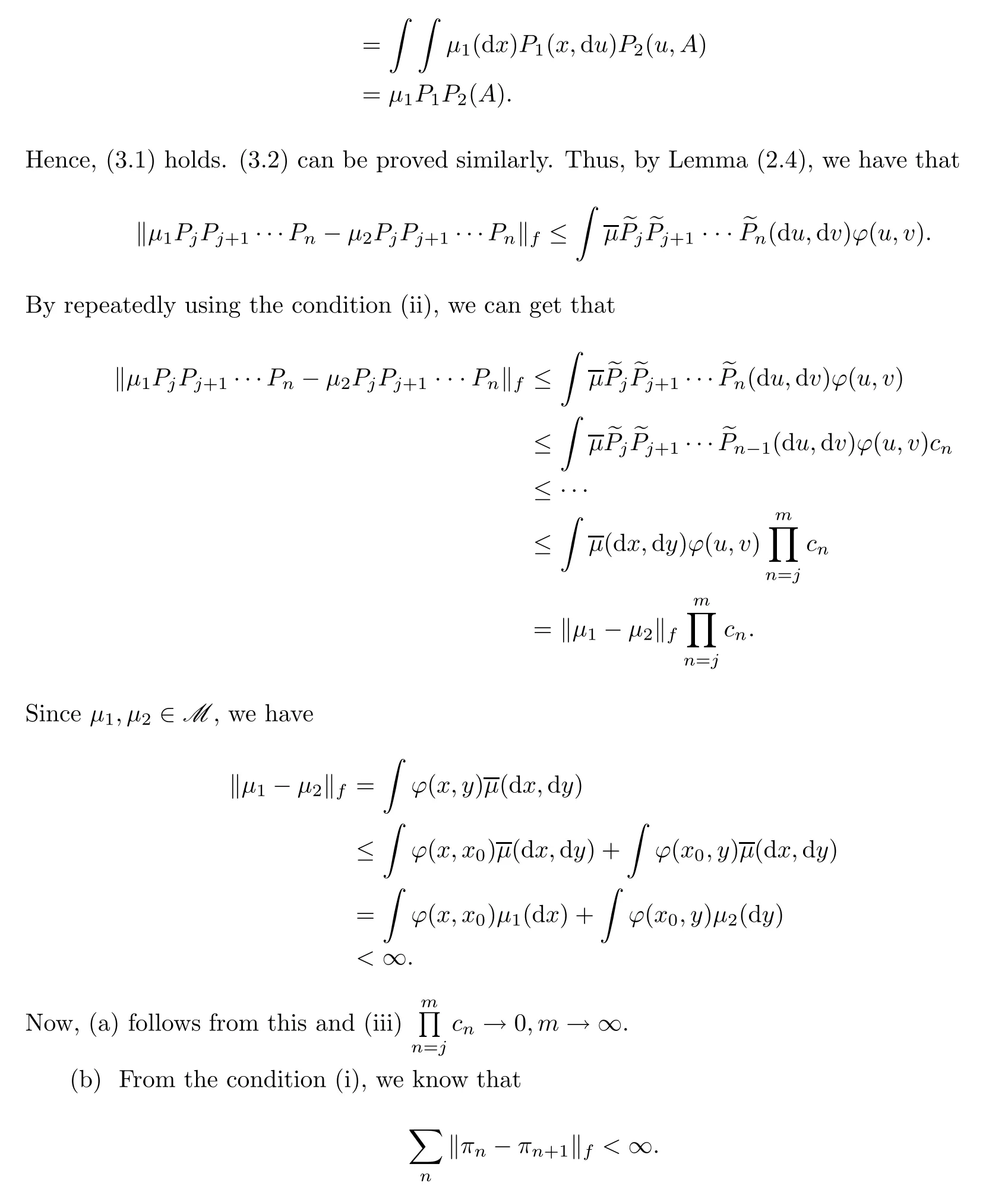
M

,W}is a complete metric space.Lemma 2.8 implies that{π:n≥1}is a Cauchy sequence on{

M

,W}.Then there exists π∈

M

such that‖π?π‖→0,n→∞.Thus(b)holds.

(c)We will prove that for?ε>0,?N∈zsuch that for n>N we have that

For any positive integer j≤n,by triangle inequality we have

Applying the condition πP=πrepeatedly to the second item above,we can deduce that

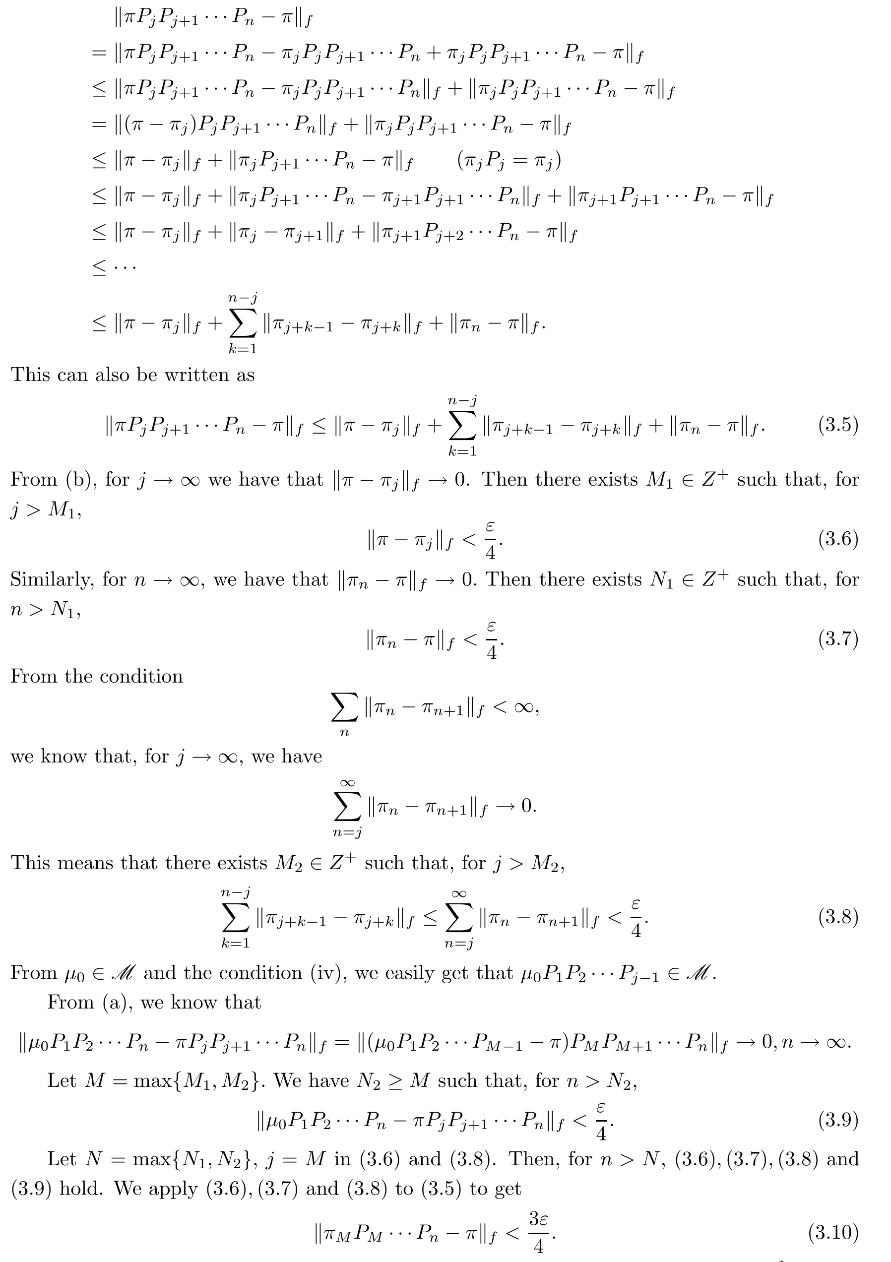
We again apply(3.9)and(3.10)to(3.4),and thus(3.3)holds.The proof of Theorem 1.2 is completed.

4 Remark on Theorem 1.2

Remark 1

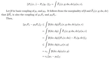
The condition(ii)can be replaced by the following:there is cuncorrelated with x,y that satis fies 0≤c≤1 such tha,t for?μ,μ∈

M

,

Remark 2

The condition(ii)can be replaced by the following:there is cuncorrelated with x,y that satis fies 0≤c≤1 such that

where ?(x,y):=d(x,y)[f(x)+f(y)],and f≥1 is a measurable function.

Remark 3

The condition(iv)can be replaced by P∈

M

.

For P∈

M

,μ∈

M

,

Thus,

Therefore,μP∈

M

.