Anyuan XIONG, Na LIU, Yujia LIU, Shulin ZHI, Linlin WU, Yongjian XIN, Yan SHI, and Yunjian ZHAN

1 National Meteorological Information Center, China Meteorological Administration, Beijing 100081

2 Jiangxi Meteorological Observatory, Nanchang 330096

3 Anhui Weather Modification Office, Hefei 230061

ABSTRACT

Key words: machine learning, benchmark dataset, quantitative precipitation estimation, precipitation forecast

1. Introduction

Data-driven machine-learning models have been widely used in weather forecasting in recent years. Using ground-based and airborne observations, such as lightning data and observations from radar systems, aircraft, and earth-observing satellites combined with mesoscale numerical weather prediction (NWP) products, machine-learning techniques have demonstrated better forecasting results than operational forecasting for severe convective weather like thunderstorms (Perler and Marchand, 2009), cloud-to-ground lighting (Zhou et al.,2020), straight-line wind storms (Lagerquist et al., 2017),hail (Marzban and Witt, 2001; Gagné et al., 2017), tornadoes (Marzban and Stumpf, 1996), and convective initiation (Mecikalski et al., 2015). The end-to-end, deeplearning technique that has been rapidly developed in recent years, e.g., convolution neural network (CNN) models, has great potential for weather forecasting. For example, the deep-learning models of Convolutional Long Short-Term Memory (ConvLSTM; Shi et al., 2015), Trajectory Gate Recurrent Unit (TrajGRU; Shi et al., 2017),and Multi-Level Correlation Long Short-Term Memory(MLC-LSTM; Jing et al., 2019) use two- or three-dimensional (2D or 3D) gridded data of previous radar reflectivity to predict the intensity of radar echoes (or precipitation) in the subsequent 0–2 hours. Compared with traditional radar extrapolation technology, these models show much better forecasting skills. The threat score(TS) of forecasts of severe convective weather like thunderstorms, heavy precipitation, hail, and gales by the CNN model, which uses physical quantities derived from NWP products as input, is well above the TS of forecasts by meteorologists in operational service (Zhou et al., 2019).

Data-driven machine learning, especially deep learning, is mostly based on labeled training datasets. The relationship between the predicted and predictors can be obtained from historical datasets, serving as the basis for developing forecast models for target variables. The larger the sample size of the training dataset, the more complete the knowledge learned by the model. Therefore, a high-quality, large-sample, and labeled training dataset is the key issue in machine learning. The construction of a training dataset takes great effort, which is financially costly and time-consuming, especially when the training samples need to be annotated by humans. For example,ImageNet (Su et al., 2012), developed at Princeton University, contains more than 14 million annotated 2D images in 21,841 synonym sets. Each image is manually labeled by using the Amazon Mechanical Turk platform.After its release to the public in 2020, ImageNet has been widely applied. It has been the standard dataset (Russakovsky et al., 2015) of the International ImageNet Large Scale Visual Recognition Challenge since 2010,greatly promoting the international development of artificial intelligence image recognition. The xBD dataset for building locations and damage assessments (Gupta et al.,2019) contains 22,068 images from the WorldView-3 satellite, with a spatial resolution of 0.3 m, and 19 different categories of labeled events, e.g., earthquakes, floods,wildfires, volcanic eruptions, and car accidents. It is one of the largest and highest quality public datasets of highresolution satellite imagery. Using this dataset for machine-learning training, we can effectively identify building damages due to various disasters and evaluate economic losses based on satellite remote-sensing data(Weber and Kané, 2020).

Severe convective weather forecasting has been made progress in China since the 1950s (Zhang et al., 2020). In spite of this, 0–6-h nowcasting of precipitation has always been a challenge because of the spin-up problem in NWP (Sun et al., 2014). Traditional methods for precipitation nowcasting are based on various radar-echo extrapolation algorithms, such as thunderstorm identification,tracking, analysis, and nowcasting (Dixon and Wiener,1993). However, weather systems are characterized by nonlinear features and large variabilities, with extrapolation algorithms often failing when weather systems change drastically. In recent years, scientists have begun to apply machine-learning techniques for precipitation nowcasting. For example, the deep recurrent neural network was used for 0–2-h precipitation nowcasting based on previous radar echoes (Shi et al., 2015, 2017; Jing et al., 2019). Due to the lack of ground-based precipitation information, label data in a training dataset can only be radar echoes. Therefore, models can only predict radar echoes, and the predicted radar echo intensity (radar reflectivity) needs to be converted into precipitation.However, large uncertainties exist in quantitative precipitation estimation (QPE) due to uncertainties of the parameters used in theZ–Rempirical relationship between radar reflectivity (Z) and ground precipitation (R)(Foresti et al., 2019). For this reason, when applying deep-learning techniques for ground precipitation forecasting, label data in the training dataset should be ground precipitation data having the same spatiotemporal attributes as the predictands. In addition, it is not enough to use radar echoes from an earlier time as the only predictor in a machine-learning model because environmental conditions have important impacts on the occurrence and development of weather systems conductive to precipitation. Many studies that attempt to apply deep learning for weather forecasting use multi-source data,especially the integrated dataset of radar observations and NWP products. For example, Zhang et al. (2019) derived a physical quantity based on Doppler weather radar reflectivity and outputs of the variational Doppler-radar assimilation system, which was then used to train a CNN model for 30-min nowcasting of convective thunderstorms. It is necessary to include multi-source information that has impacts on the target variable in machinelearning training data.

To encourage and promote the development of artificial intelligence models for specific applications, it is very important to establish a benchmark dataset. Different models can be developed and compared based on the same benchmark dataset and unified evaluation metrics.For example, the ECMWF released WeatherBench in 2020 (Rasp et al., 2020), a machine-learning benchmark dataset for weather and climate simulations and forecasting. This dataset contains 8 variables at 13 isobaric levels and 6 surface variables based on the ERA5 global reanalysis product, which can be used for the training and testing of deep-learning models. Based on this benchmark dataset, complex and diverse deep neural network models can be developed for weather forecasting with various lead times. Forecasting performances can be compared and evaluated by using the benchmark Weather-Bench.

The present study develops a benchmark dataset that can be applied to machine learning for minute-scale quantitative precipitation estimation and forecasting(QpefBD). The dataset contains Doppler radar products for 3185 heavy convective precipitation events in heavyrainfall-prone areas of eastern China and numerical model outputs or derived physical quantities that are closely related to ground precipitation. Ground precipitation data whose spatiotemporal resolutions are consistent with those of the radar products are used as label data in Qpef-BD. Several commonly used verification metrics are implemented as the evaluation benchmark. Section 2 describes various data contained in QpefBD and the procedures to process these data. Section 3 gives the benchmarks for QPE and quantitative precipitation forecast(QPF) evaluation based on commonly used methods.Section 4 describes three application scenarios of the dataset. The availability of the dataset is given in Section 5. Conclusions and summary are provided in Section 6.

2. Description of the dataset

The benchmark QpefBD dataset mainly supports precipitation estimation and quantitative precipitation nowcasting based on weather radar observations. QpefBD contains Doppler weather radar products, atmospheric condition parameters (ACP), and two types of ground precipitation data as labels within the time windows of 9832 convective heavy rainfall events (CHREs) that occurred from April to October 2016–2018 in 6 provinces of China (Hubei, Hunan, Anhui, Jiangxi, Zhejiang, and Fujian). These CHREs are single-station CHREs (called CHRE-S), obtained based on 60-min precipitation at a station (details can be found in Section 2.1). The time window of a CHRE-S is defined as 2 h before the event start time to 2 h after the event end time. The time window of heavy precipitation event is extended by 4 h mainly because: (1) the sample size of training data can be increased, and (2) a heavy precipitation event is a continuous mesoscale weather process. The sampled data within the extended time window can more completely describe the genesis, development, and dissipation of a weather system.

Due to the importance of radar data in precipitation estimation and forecasting, each CHRE-S selects an S-band weather radar station adjacent to the ground station and uses this radar station as the center of the spatial coverage to obtain label data, radar products, and ACP within a certain spatial range. In this way, different CHRE-Ss may choose the same radar as their spatial center to obtain data, resulting in large amounts of duplicate data. In QpefBD, duplicate data are processed. For different CHRE-Ss with the same radar selected, if there are overlaps in their time windows, the CHREs of these different stations are combined into one single CHRE (called CHRE-R). A single CHRE-R may contain multiple CHRE-Ss. Eventually, 3185 CHRE-Rs were obtained.The time window for more than 80% of the CHRE-R cases is within 4–8 h, and the maximum time window can be up to 60 h.

Weather radar products include eight radar variables at about 6-min intervals in the time window of the event.ACP are physical variables or derived quantities obtained from the ERA5 reanalysis product (Hersbach et al., 2020), representing atmospheric dynamic and thermodynamic conditions during a CHRE. Two types of ground precipitation data as labels, i.e., 6-min rainfall intensity and the area covered by heavy rainfall, are the label data (or true values) used in machine learning. Sections 2.2, 2.3, and 2.4 provide detailed descriptions of the data. Figure 1 shows examples of 2D patterns of several variables contained in a sample.

All data are saved as 2D slab data with equal longitudinal and latitudinal grid spacings. The horizontal resolution of radar and ground precipitation data is 0.01°, and the temporal resolution is 6 min. The background weather data (i.e., ACP) in 0.25° × 0.25° grids have a temporal resolution of 1 h. To facilitate data processing by general machine-learning platforms, all 2D gridded data are stored in the Numpy binary format that can be directly read by the Python programming language.

Table 1 lists the number of CHRE-Rs and the number of samples for each individual year.

The number of samples for a single CHRE-R refers to the number of data collection times within the time window of the CHRE-R. A sample is generally taken every six minutes. If the time window of a CHRE-R is 5 h, the number of samples for this CHRE-R should be 50. Each sample data include radar products, atmospheric condition parameters, and labels of ground precipitation data.The former two are input data (or predictors) for a machine-learning model, and the latter are the labels for the inputs of the model.

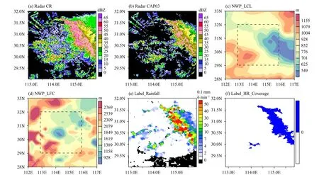
Fig. 1. Examples of 2D patterns of several variables contained in a sample from a heavy precipitation event [2337 BT (Beijing Time) 18 to 1226 BT 19 June 2016]: (a) composite radar reflectivity and (b) radar reflectivity at an altitude of 3 km in Wuhan at 0803 BT 19 June, (c) lifted condensation level and (d) level of free convection at 0800 BT 19 June, (e) 6-min precipitation (label data), and (f) heavy rainfall area (label data) at 0803 BT 19 June. The dashed, black squares in (c) and (d) show areas where radar data and label data are consistent.

Table 1. The number of CHRE-Rs (NCHRE-R) and the number of samples (Nsample) for each year

When training a machine-learning model, the datasets used are usually divided into a training dataset and a testing dataset. The former is used for model training to determine various model parameters, and the latter is used as independent data for model performance evaluation.We use the sampled data collected in the six provinces in May, July, and September 2018 as testing data and the remaining data as training data. The testing data contain samples from different seasons to test seasonal differences in the model performance. The training data contain 2544 heavy precipitation events, and the number of samples is 189,039. There are 641 heavy precipitation events and 42,939 samples in the testing dataset, accounting for 18.5% of the total number of samples. The reference benchmark for the model performance evaluation given in Section 3 is calculated based on the testing data.

The ground precipitation data and radar observations are provided by the National Meteorological Information Center, China Meteorological Administration. The ERA5 reanalysis product is downloaded from the ECMWF Copernicus Climate Change Service (https://cds.climate.copernicus.eu/).

2.1 Severe convective precipitation events

QpefBD contains CHREs that occurred in Hubei,Hunan, Anhui, Jiangxi, Zhejiang, and Fujian provinces from April to October 2016–2018. These provinces are located in eastern and central China, regions prone to heavy convective precipitation. Heavy rainstorms and floods in the summertime pose a major threat to local economic development and human safety.

Short-term heavy precipitation usually refers to precipitation events with hourly rainfall amounts equal to or greater than 20 mm. To match the temporal resolution of radar observations, 1-min precipitation observations collected at all 491 national automatic weather stations in the 6 provinces are used to calculate 6-min precipitation information in accordance with the radar observation period. Operational quality control was conducted on the 1-min precipitation observations, and those data flagged as incorrect or suspicious were excluded. Here, a severe precipitation event (CHRE-S) is identified when a 60-min rainfall amount is greater than or equal to 20 mm at a single station. A sliding calculation is applied to obtain 60-min precipitation amounts at each individual station based on time series of 1-min precipitation amounts at each station. The start time of a heavy precipitation event at a station is the beginning minute when the 60-min precipitation amount starts to meet the criterion (≥ 20 mm),and the end time of the event is the ending minute when the last 60 minutes of cumulative precipitation (≥ 20 mm) ends.

The study area in China is frequently affected by western Pacific typhoons. Single-station heavy convective precipitation events caused by typhoons are excluded from QpefBD. Here, typhoon-induced heavy precipitation refers to the precipitation that occurs within a radius of 400 km around the typhoon center. Typhoon track data are extracted from the typhoon best-track dataset produced by the Shanghai Typhoon Institute of the China Meteorological Administration (CMA-STI Best Track Dataset for Tropical Cyclones over the western North Pacific; Ying et al., 2014), available at http://tcdata.typhoon.org.cn.

Figure 2 shows the spatial distribution of stations with CHRE-S in the 6 provinces from April to October 2016–2018 and the number of heavy precipitation events at each station.

2.2 Weather radar data

For each individual CHRE, the weather radar station with the most complete data and closest to the station where the CHRE occurred is first identified. All 6-min radar data collected at this radar station during the time window of the CHRE are then obtained. Quality control is performed to remove various non-precipitation echoes,including noise (outlier) filtering, radial interference recognition, ground/super-refraction echo recognition,ocean-wave echo recognition, and clear-sky echo elimination. The quality-control algorithms used are referenced in the literature (Liu et al., 2007; Leng et al., 2012; Tan et al., 2013; Wen et al., 2016). Multiple physical quantities are obtained from the quality-controlled radar data to represent different meteorological features. The benchmark dataset developed in the present study contains eight products that are closely related to surface precipitation (Table 2). The eight radar quantities listed in Table 2 have clear physical significance and are the most frequently used products in meteorological operations. They are well related to the spatial distribution of and variation in surface precipitation and are useful for identifying heavy precipitation weather conditions (Yu et al.,2006).

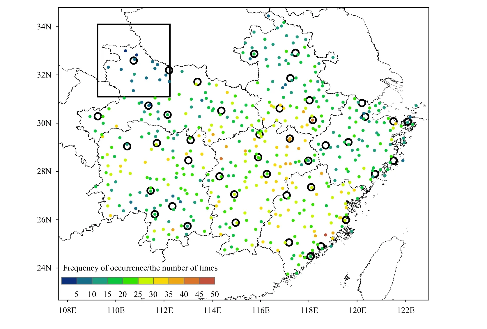
Fig. 2. Locations of national-level surface stations (solid, colored dots) and weather radars (open, black circles). Rainfall observations made at these surface stations are used to determine heavy precipitation events. The colors show the occurrence frequencies of single-station, short-term,heavy precipitation events from 2016 to 2018. The black box denotes the area coverage by a single radar.

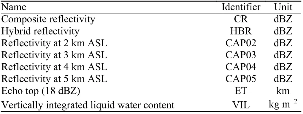
Table 2. Radar data products contained in the benchmark dataset.ASL stands for above sea level

The composite reflectivity (CR) is the maximum reflectivity of scans at all elevations, representing the strongest echo in the 2D space obtained by the radar. If the strongest echo occurs at a lower altitude, ground precipitation can be well reflected by radar echoes. The hybrid reflectivity (HBR) is the echo intensity observed by the radar at the lowest elevation angle above the terrain height, which can well reflect surface precipitation (Xiao et al., 2008) and is the main radar product used in QPE.Radar reflectivities at the four altitude levels between 2 and 5 km shown by the constant altitude plan position indicator (CAPPI) at each level are obtained by 3D interpolation of radial data at different elevation angles using the algorithms proposed by Xiao and Liu (2006). Only CAPPIs at these 4 levels are selected here because echoes between 2 and 5 km are more closely associated with ground precipitation. The higher-level CAPPI has a bright band of echoes due to solid precipitation particles,which may contaminate the precipitation echo signal.CAPPIs below 2 km are mostly affected by the side-lobe echo, ground clutter, and the super-refraction echo. For example, the CAPPI at the 3-km height is commonly used to analyze the climatological characteristics of convective storms (Chen et al., 2014). The echo top (ET) is the highest altitude that a target with a reflectance factor above 18 dBZ can be detected by radar. ET products can be used to detect storms (Yu et al., 2006). The 18-dBZ value is approximate to the radar echo intensity that may generate surface precipitation. It is generally used as the default value for echo-top-height products in operational nowcasting systems in the United States and China. The vertically integrated liquid water content (VIL) is the sum of equivalent liquid water contents derived from radar reflectivities at each scanning elevation angle. For this calculation, it is assumed that all reflectivities are caused by liquid water drops (Yu et al., 2006).

The radar product is gridded data of equal latitudinal and longitudinal intervals, covering a rectangular area of 3° × 3° centered on the radar station with 301 × 301 grids, and the resolution is 0.01° × 0.01°.

The benchmark dataset contains data collected by 43 weather radars. All 43 radars are S-band Doppler weather radars with a wavelength of 10 cm. Figure 2 shows the locations of the 43 radar stations and an example of area coverage by a single radar.

2.3 Atmospheric condition parameters

Short-term, heavy rainfall is generally a weather phenomenon that occurs in mesoscale convective systems,but not all mesoscale convective systems can generate heavy rainfall. Only under favorable weather conditions can mesoscale systems easily develop and produce strong surface precipitation. Zhang et al. (2012) reported that the background weather conditions for the occurrence and development of strong mesoscale convective systems include four elements: water vapor, static instability, uplift, and vertical wind shear. Yu and Zheng (2020)systematically reviewed the environmental conditions of static instability, moisture, and lifting for severe convective weather. A diagnostic analysis of the environmental conditions for the occurrence and development of convection based on radiosonde data or numerical model products is helpful for forecasting short-term, severe convective weather. For example, Doswell et al. (1996) proposed an “ingredients-based” method to diagnose and analyze three types of weather conditions, including water vapor, convective instability, and uplift for heavy precipitation events. This method was eventually used for the operational forecasting of heavy rainstorms in China(Tang et al., 2010; Zhang et al., 2010).

In order to consider the weather conditions for the occurrence and development of heavy rainfall during an operational forecast, weather-condition data are needed at the time of the forecast and the previous period as input for the machine-learning model. QpefBD contains 27 physical parameters, i.e., ACP, describing atmospheric water vapor, static instability, and dynamic lifting conditions (Table 3). The parameters are closely related to weather conditions associated with the occurrence and development of heavy rainfall and have explicit physical significance. ACPs are calculated based on the ERA5 reanalysis product, which has a spatial resolution of 0.25° and a temporal resolution of 1 h. ACPs are direct model output, while others are derived from model output at the surface and at various isobaric levels using the Sounding and Hodograph Analysis and Research Program in Python (SHARPpy) software package (Blumberg et al., 2017). SHARPpy can be available at https://github.com/sharppy/SHARPpy.

All ACPs are 2D rectangular gridded data, with spatial and temporal resolutions the same as those of ERA5.Considering the possible impacts of weather conditions around the forecast target area (i.e., the area defined by radar products and label data) on precipitation in the target area, the spatial range of ACP is a 5° × 5° rectangular area. This is larger than the label data area, and its center point is the grid point closest to the radar station.ACPs are used as input to the machine-learning model.However, the area and resolution of ACPs are different from those of the radar products and label data, challenging the development of a machine-learning technique.

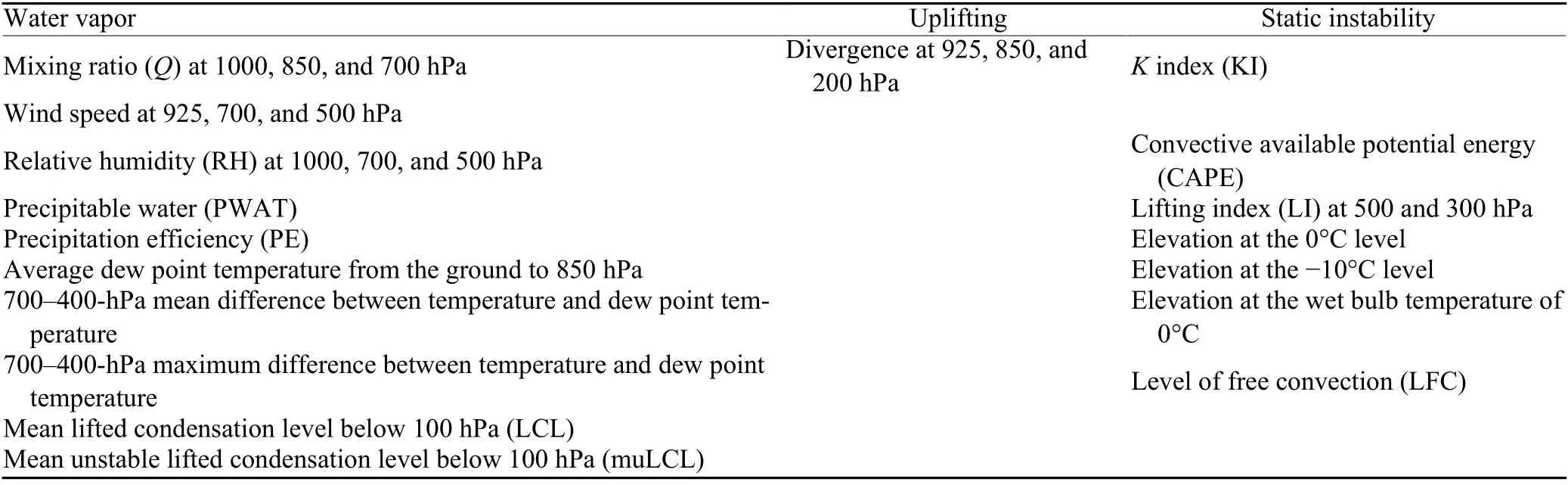
Table 3. The 27 atmospheric condition parameters contained in QpefBD

2.4 Labels

Most machine-learning methods are supervised-learning methods, i.e., each sample in the dataset needs to be given a true value (a label) representing the forecast,which is called label data. For example, in ImageNet (Su et al., 2012), each image is manually labeled (such as“motorbike” and “bicycle”). An object-recognition model can be obtained through learning and training with a large number of labeled samples. In the field of geoscience, the dataset often contains huge amounts of samples, while labeling these samples requires complicated professional skills and a great deal of time. For this reason, Reichstein et al. (2019) listed the lack of labeled datasets as one of the five major challenges in the application of artificial intelligence to geosciences. The quality of the label data is the most critical factor affecting the performance of machine-learning models.

The present study produces two types of label data,i.e., rainfall intensity data showing the spatial distribution of 6-min precipitation and heavy rainfall area data showing where heavy rainfall occurs.

2.4.1Label of precipitation intensity

For precipitation estimation and forecasting, QpefBD needs to provide an actual ground precipitation distribution for each training sample. However, it is hard to obtain “true” surface precipitation distributions. Fortunately, 15,652 ground precipitation observation stations are densely distributed in the area covered by this dataset (Fig. 3). These include all national-level weather stations (Fig. 2) and regional-level weather stations in the six provinces. The temporal resolution of the precipitation observational data is 1 min, which can be used to derive precipitation data at 6-min intervals, matching the time period of a complete radar-volume scan.

To obtain label data consistent with the temporal and spatial attributes of the main input data (i.e., radar products), ground precipitation observations collected at weather stations need to be remapped to 0.01° × 0.01°grids. Here, the piecewise inverse distance squared weighted interpolation method is used, expressed as

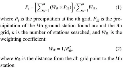
The search radii are 1, 5, and 10 km. If stations can be found within a 1-km radius, the labeled value is the precipitation recorded at the station closest to the grid point.If no valid station can be found within a 1-km radius, the search radius is sequentially expanded to 5 and 10 km,and Eq. (1) is used to calculate precipitation at the grid point. If no station is found within 10 km, precipitation at that grid point is given the value of ?9, indicating a missing value. Multiple search radii are used here mainly for the purpose of preserving as much as possible real precipitation information from the nearest neighboring area of the grid, making sure heavy precipitation at stations close to the grid will not be underestimated due to interpolation. As a result, the gridded precipitation data interpolated from observations retain extreme precipitation information observed at the stations.

The label data cover a 2D rectangular area with the same size as that of radar products, with the center of the area corresponding to the position of the radar station.The temporal and spatial resolutions of the dataset are the same as those of radar products.

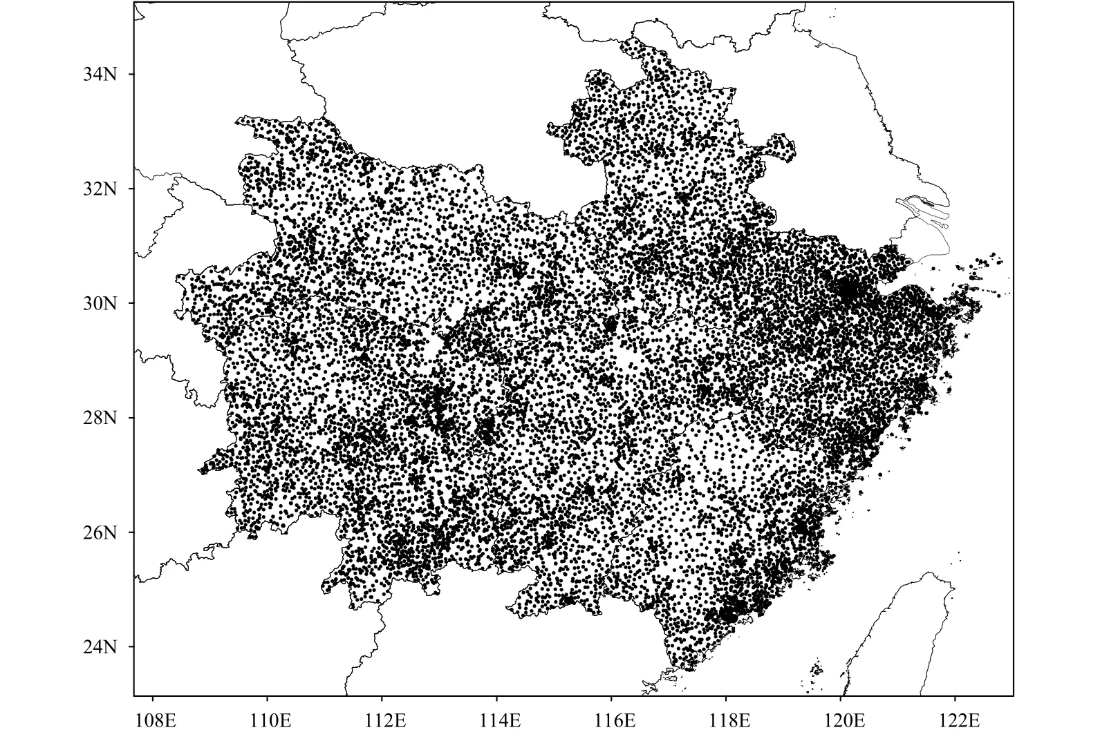
Fig. 3. Distribution of ground precipitation observation stations.

Since there are no ground precipitation observations in some uninhabited mountainous areas and over large water bodies, label data still contain many missing values,affecting how machine-learning models learn. To reduce the proportion of missing values, missing values are filled by zeros at those grids identified as having no precipitation based on the CR in the same area and the hourly, 5-km resolution precipitation product called CMA Multi-source merged Precipitation Analysis System (CMPAS), which is a product fusing three sources of observations, namely, observations from radar, satellite,and ground rain gauges (Pan et al., 2015). The criteria for identifying non-precipitation grids are: (1) CR is valid but no more than 10 dBZ, and (2) when criterion (1) cannot be satisfied, CMPAS’s 1-h precipitation is less than 0.1 mm. After the above processing, the proportion of missing values in the label data is reduced from 21.68%to 5.97%, indicating that the amount of missing data has been greatly reduced. Figure 4 shows the frequency distribution of the proportion of missing values before and after the processing.

2.4.2Label of heavy precipitation areal coverage

Based on radar reflectivity data at various elevation angles, a storm cell size exceeding a given threshold is identified by using the storm cell identification and tracking algorithm (Johnson et al., 1998). It is applied to all storm cells at all elevation angles, and results are combined by a union operation. All storm cells in the union are projected onto the grids in turn, and all the grid points surrounded by the storm cells can be used to denote storm cells. The threshold of the echo intensity is 35 dBZ. Heavy precipitation areas are mainly labeled based on the radar storm cell size and 6-min accumulated precipitation at stations. If the 6-min precipitation amount is greater than or equal to 3 mm at a single station within the storm cell, all the grid points covered by the storm cell are given the label 1. If no 6-min precipitation amount is greater than or equal to 3 mm at any station within the storm cell, then all the grid points covered by the storm cell are given the label 0. If there is no observation station within the storm cell, the grid points covered by the storm cell are all given the missing value label,i.e., ?9. Grid points outside the storm cell are labeled 0 regardless of whether there is heavy precipitation or not.

The spatial range and spatiotemporal resolutions of the label data of heavy precipitation areal coverage and precipitation intensity are the same.

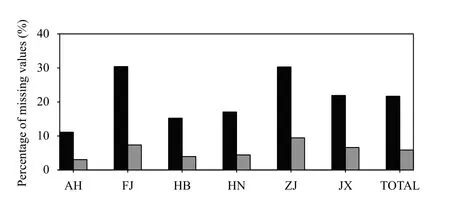
Fig. 4. Percentage of missing values in the precipitation intensity label data before (black bars) and after (gray bars) their filling for the six provinces, i.e., Anhui (AH), Fujian (FJ), Hubei (HB), Hunan (HN),Zhejiang (ZJ), Jiangxi (JX), and the average (TOTAL).

3. Reference benchmark for performance evaluation of a machine-learning model

To build a machine-learning model based on QpefBD,the performance of the model needs to be evaluated. To provide a comparable reference benchmark for the evaluation of different models developed by different research-and-development institutions, QpefBD provides several unified evaluation metrics. In addition, a few commonly used methods or methods used in operational weather services are applied to precipitation estimates and forecasts. Skill scores are given, serving as the benchmark reference. Precipitation estimation and forecasting methods include radar quantitative precipitation estimation, persistence forecasting, and optical flow extrapolation based on semi-Lagrangian extrapolation.

3.1 Evaluation metrics

The following metrics are used to evaluate the model performance on precipitation estimation and forecasting:

(1) Root-mean-square error (RMSE)

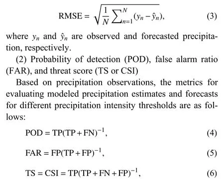
where TP (true positive) is the number of forecasts and observations that are both true, FN (false negative) is the number of false forecasts and true observations, and FP(false positive) is the number of true forecasts and false observations.

3.2 QPE based on the Z–R relationship

Calculating precipitation based on the exponential relationship betweenZandR(i.e., theZ–Rrelationship) is an effective method to quickly obtain the distribution of surface precipitation in meteorological services. The algorithms used in operational weather services are implemented in the present study to estimate hourly precipitation (QPE) using the testing dataset. The steps taken are as follows.

(1) Calculate the first guess of 1-h precipitation (R):About 10 hybrid reflectivity data samples in the previous hour are used to calculate the precipitation rate based on theZ–Rrelationship, which is expressed asZ=aRb. The sum of the results is the 1-h QP estimate. Here,Z(mm6m?3) is the radar hybrid reflectivity,R(mm h?1) is the estimated precipitation,a= 300, andb= 1.4.

(2) Use the 1-h precipitation data collected at weather stations to correct the hourly precipitation,R, first guess:Assuming that there arenweather stations in the area covered by the radar, and the arithmetic average of 1-h precipitation at these stations isRg, the average precipitation first-guess estimate at thengrids closest to the stations isR. The weather stations used include all the stations shown in Fig. 3. The correction factor isL=RgR?1.

The corrected precipitation estimate is QPE =L×R.Hourly QP estimates during the period covered by the testing dataset can then be obtained.

One-hourly precipitation values are first derived from the 6-min precipitation information contained in the label data of precipitation intensity and taken as the true values. Forecast skill scores of RMSE, POD, FAR, and TS for different precipitation intensity intervals of the radar QPE (i.e., 0, ≥ 0.1, ≥ 5, ≥ 10, ≥ 15, and ≥ 20 mm h?1) are finally calculated.

Appendix A presents detailed results, which are used as the baseline for evaluating the performance of radar precipitation estimation models.

3.3 Persistence forecast

A persistence forecast assumes that the forecasted quantity at all forecast times is the same as the quantity at the initial time of the forecast. Here, persistence refers to Eulerian persistence instead of Lagrangian persistence.Persistence forecast results are often used as a benchmark to evaluate the forecast skills of other methods.

Based on the testing dataset, consecutive persistence forecasts of 6-min ground precipitation within the time window of each heavy precipitation event are carried out.Statistics of skill scores for the model performance are calculated by using the label data of precipitation intensity as true values.

Appendix B presents detailed results.

3.4 Forecast by optical flow extrapolation

The optical flow method assumes that the moving target (such as precipitation) has Lagrangian persistence(Liu et al., 2015). The 2D fields of the target at two consecutive times are used to calculate the advection field(i.e., the optical flow field) then extrapolated to the target position at the forecast time. There are many algorithms for optical flow extrapolation. The present study uses the algorithm called the real-time optical flow by variational method for echoes of radar (ROVER) developed at the Hong Kong Observatory (HKO). Shi et al.(2015) provide the code, with details found at https://github.com/sxjscience/HKO-7.

Using the 6-min precipitation at the start time of the forecast and the previous time in the testing dataset, the optical flow extrapolation method is applied to predict precipitation in the subsequent 20 consecutive 6-min periods (6–120 min). Statistics of the performance for these forecasts are calculated by using the label data of precipitation intensity as true values.

Appendix C presents detailed results.

4. Dataset application scenarios

QpefBD can be used for minute-scale radar precipitation estimations and 0–2-h precipitation nowcasting.Three application scenarios are given next. Section 4.4 gives a few suggestions for further data processing.

4.1 Radar-based QPE (6-min and 1-h precipitation)

Based on the radar precipitation echo intensity and the physical relationship between the echo intensity and ground precipitation (i.e., theZ–Rrelationship), a radarbased QP estimate can be obtained. This has been the commonly used method in operational weather services in recent decades. Data-driven machine-learning technology has the potential to improve precipitation estimation. Using QpefBD, a machine-learning model can find the connection between radar observations and ground precipitation. For example, a deep neural network can learn the complicated nonlinear relationship between 2D radar products and 2D ground precipitation from the training dataset and directly output the spatial distribution of 2D ground precipitation. Input data for the deeplearning model include one or more of the eight radar products listed in Table 2. They are used as the model’s multi-channel, 2D spatial data. Since the 2D spatial samples in the training dataset contain data from different regions and seasons and also different radars. Factors such as region, terrain, season, and diurnal variation can thus be added to input data to consider their possible influences on precipitation. This will improve the accuracy and the generalization ability of the model. However, this will also increase the complexity of the model, requiring more computing resources. The model outputs are 2D gridded datasets of 6-min ground precipitation (or precipitation rate), covering the same spatial area as the radar products.

4.2 0–2-h precipitation nowcasting at the minute scale

Zero-to-two-hour nowcasting of surface precipitation is a challenging issue in operational weather forecasting.It is also of interest to other scientific research efforts.QpefBD provides a standard dataset for precipitation nowcasting on a minute scale based on machine learning.We recommend applying QpefBD in deep neural network models, such as the recurrent neural network and its various derivative models (e.g., LSTM and GRU) that have the ability to deal with time series of prediction. Using the large-capacity training samples provided by QpefBD, such as the sequences of radar products at the initial time of the forecast and the previous periods, plus background ACP data at the time of the forecast and the“true values” of ground precipitation represented by label data, a deep machine-learning model can be established. The neural network model can learn (1) the temporal variation regularities of precipitation from previous radar products and (2) the relationship between weather conditions and ground precipitation from the ACP physical quantities at the forecast time, eventually realizing 6-min precipitation forecasting.

4.3 Interpretation of precipitation based on model forecast products

The model output can be converted into a forecast of ground elements by establishing relationships between the forecast products of numerical weather models and ground elements (e.g., conventional elements like temperature, humidity, and wind, or strong convective weather phenomena, such as storms, heavy precipitation,and hail). Traditional statistics-based model interpretation technology can hardly determine the nonlinear relationships between model products and ground elements[e.g., the Model Output Statistics (MOS) method]. Datadriven machine-learning technology offers a new approach. A machine-learning model is established by using a large number of training data samples. The relationship between model output variables and ground forecast variables can then be obtained regardless of whether the relationship is linear or nonlinear. At present, a large number of results have been generated by using machinelearning technology. For example, 57 characteristic quantities closely related to the occurrence of thunderstorms are obtained from the Swiss mesoscale weather model called aLMo and used as input to the sampling machine-learning model called AdaBoost. The model is then used to predict the occurrence probability of thunderstorms, generating better predictions than those of an expert system (Perler and Marchand, 2009). Whether lightning will occur or not on each grid point in the Korean Peninsula can be predicted by using the ECMWF global forecast products at 3-h intervals (Han et al.,2017). Zhou et al. (2019) used a deep network model to establish the relationship between the output of the US NCEP Global Forecast System (GFS) model and the occurrence of severe convective weather (i.e., thunderstorms, heavy precipitation, hail, and high convective winds) on the ground, realizing the potential forecast of strong convective weather on the ground based on the GFS real-time forecast.

QpefBD contains 6-min surface precipitation distributions within the time window of heavy precipitation events and 27 hourly physical quantities produced by numerical models. The deep neural network model can then be used to determine the relationship between ACP and ground precipitation based on this dataset. Since the label data of surface precipitation are 6-min precipitation amounts and ACP are hourly data, label data need to be converted into hourly data, with the target of the forecast being the hourly precipitation field. Also, the spatial resolution of the ground precipitation data is 0.01°, whereas the spatial resolution of ACP is 0.25°. The spatial ranges of the two datasets are inconsistent. The area of the labeled data is within the area covered by ACP, which has a larger spatial area than the label data. How to establish the spatial mapping relationship between the two datasets poses a challenge to the development of deeplearning models.

4.4 Suggestions for further data processing

The radar products in QpefBD have some non-valid data due to ground clutter and other non-precipitation echoes. These are denoted by the integers ?32,768 for missing data and ?1280 for no valid echoes. When radar products are used as input to the deep-learning model,these data should be preprocessed. For example, invalid values in the CR, HBR, and CAPPI products could be replaced with 0 dBZ so that surface precipitation is not produced. Similarly, label data have some missing data due to the lack of enough ground precipitation stations,denoted by ?9. These missing data cannot be involved in the calculation of loss during model training.

When machine-learning models are trained, input data and label data need to be normalized during data preprocessing due to inconsistencies in the units of measure between the different input data and between the input data and output data.

Topography has an important influence on the occurrence and development of surface precipitation. Machine-learning models for precipitation estimation and forecasting often include topographic features (e.g., elevation, slope, and aspect) as important input data, e.g.,Google’s precipitation forecasting model (S?nderby et al., 2020). We suggest that for precipitation estimation and forecasting models developed for regions with complex topography, topographic and geographic factors could be added to the input of the model that uses radar products. The topographic and geographic data should be processed with the same spatial attributes as the radar products. The merging of topographic and geographic data with other input data could improve the forecasting performance of the model, thus enhancing the generalization ability of the model to different regions.

5. Data availability

The dataset developed in this study is open to domestic users in China for free, available at http://10.1.64.154/idata/web/data/index. It can be used for scientific research and operational services for the public welfare.Users wishing to use this dataset for commercial purposes must obtain permission from the owner of the dataset, i.e., the National Meteorological Information Center.The dataset will be updated over the next year to cover more time periods, e.g., 2019 and 2020, and more regions, e.g., 11 more provinces.

6. Summary

The present study has developed a benchmark dataset,i.e., QpefBD, which can be used in machine-learning models for ground precipitation estimation and forecast.The basic characteristics of the dataset are as follows.

(1) Data samples are taken from 3185 heavy precipitation events that occurred during March–October of 2016–2018 in 6 provinces in central and eastern China.In total, there are 228,809 samples.

(2) The dataset includes Doppler weather radar data,ACP, and two kinds of labels (precipitation intensity and heavy precipitation area). The radar data contain eight radar products closely related to the occurrence and development of ground precipitation. The ACP data are from ERA5 hourly reanalysis data and their derived physical quantities. The label data have the same spatiotemporal attributes as the radar data, i.e., a horizontal resolution of 0.01° and a temporal resolution of 6 min.

(3) The samples contained in the dataset are two-dimensional gridded raster data with equal latitudinal and longitudinal intervals, directly usable for the training of machine-learning models, especially the deep-learning models.

The present study provides metrics for the evaluation of machine-learning-model performance. The results of model evaluation based on these metrics can serve as the baseline for the performance evaluation of machinelearning models using this dataset.

QpefBD can be widely used in scenarios such as single-station Doppler weather radar quantitative precipitation estimation, minute-scale precipitation nowcasting,and precipitation forecast interpretation based on products from numerical weather models. We believe that extensive application of this dataset can effectively promote collaborative studies in various atmospheric science fields, upgrade the application of artificial intelligence in the meteorological sciences, and improve ground precipitation forecasts (especially short-term heavy precipitation forecasts). We also hope that more artificial intelligence scientists will work with experts in the atmospheric sciences to develop algorithms and models that can effectively solve problems specifically associated with the atmospheric sciences.

Appendix A: The baseline performance of operational radar QPE

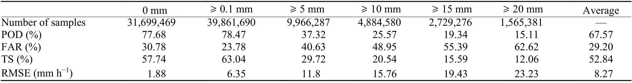
Table A1. RMSEs of radar precipitation estimates based on the Z–R relationship

Appendix B: The baseline performance from the persistence forecast of rainfall

Table B1. RMSEs of 6-min precipitation persistence forecasts

Fig. B1. Threat scores (TSs) for the persistence forecasts of 6-min precipitation with different magnitudes [0, ≥ 0.1, ≥ 1, ≥ 2, and ≥ 3 mm (6 min)?1] as a function of forecast lead time.

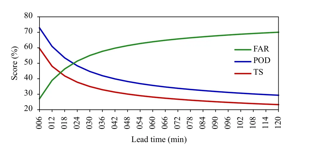
Fig. B2. Probability of detection (POD), false alarm ratio (FAR), and threat score (TS) for persistence forecasts of 6-min precipitation as a function of forecast lead time.

Appendix C: The baseline performance of the rainfall forecast using optical flow extrapolation

Table C1. RMSEs of 6-min precipitation forecasts generated by the optical flow extrapolation method

Fig. C1. Threat scores (TSs) for forecasts of 6-min precipitation with different magnitudes [0, ≥ 0.1, ≥ 1, ≥ 2, and ≥ 3 mm (6 min)?1] as a function of forecast lead time using the optical flow extrapolation method.

Fig. C2. False alarm ratio (FAR), probability of detection (POD), and threat score (TS) for consecutive forecasts of 6-min precipitation as a function of forecast lead time using the optical flow extrapolation method.