Sunshun YuanLing ZhuCheng LiuHan Quand Zhou Fan

1 Shanghai Astronomical Observatory,Chinese Academy of Sciences,Shanghai 200030,China; yss@shao.ac.cn, lzhu@shao.ac.cn

2 Department of Astronomy and Space Sciences,University of Chinese Academy of Sciences,Beijing 100049,China

3 National Astronomical Observatories,Chinese Academy of Sciences,Beijing 100101,China

Abstract We construct a multiple-population discrete axisymmetric Jeans model for the Andromeda (M31) galaxy,considering three populations of kinematic tracers: 48 supergiants and 721 planetary nebulae (PNe) in the bulge and disk regions,554 globular clusters extending to ～30 kpc,and halo stars extending to ～150 kpc of the galaxy.The three populations of tracers are organized in the same gravitational potential,while each population is allowed to have its own spatial distribution,rotation,and internal velocity anisotropy.The gravitational potential is a combination of stellar mass and a generalized NFW dark matter halo.We created two sets of models,one with a cusped dark matter halo and one with a cored dark matter halo.Both the cusped and cored model fit kinematics of all the three populations well,but the cored model is not preferred due to a too high concentration compared to that predicted from cosmological simulations.With a cusped dark matter halo,we obtained total stellar mass of 1.0±0.1×1011 M⊙,dark matter halo virial mass of M200=7.0±0.9×1011 M⊙,virial radius of r200=184±4 kpc,and concentration of c=20±4.The mass of M31 we obtained is at the lower side of the allowed ranges in the literature and consistent with the previous results obtained from the H I rotation curve and PNe kinematics.Velocity dispersion profile of the outer stellar halo is important in constraining the total mass while it is still largely uncertain.Further proper motion of bright sources from Gaia or the Chinese Space Station Telescope might help on improving the data and lead to stronger constraints on the total mass of M31.

Key words: Galaxy:kinematics and dynamics–galaxies:luminosity function–mass function–Galaxy:evolution

1.Introduction

The Andromeda galaxy (M31) and Milky Way (MW) are the only two giant spiral galaxies in the Local Group.M31 is close enough that single stars’ chemical and kinematic properties are resolved,which allows studies in great detail on its structure formation history.The starlight of M31 is dominated by a disk,which is about twice as massive and with a scale length twice large as that of the MW(Boardman et al.2020).The disk of M31 is quite edge-on along the line-of-sight(LOS),the bulge region is thus not easy to observe,but it probably has a bar-shaped structure in the center region,similar to the MW(Bla?a Díaz et al.2018).M31 has a much more massive stellar halo and a significantly larger number of satellite galaxies than the MW(Ibata et al.2014;Wetzel et al.2016).The larger disk mass,halo mass,and more satellite galaxies in M31 could be scaled by its larger total mass,but could also be caused by its different formation histories compared to the MW.The giant streams in the inner halo of M31 indicate a recent major merger at ～2 Gyr ago (D’Souza &Bell2018;Hammer et al.2018),while the last massive merger in the MW is supposed to be ～10 Gyr ago with only minor mergers since then(Helmi2020;Belokurov et al.2020).Both the MW and M31 could have a total mass of 0.5?3×1012M⊙,it is still controversial which one is more massive due to uncertainties on both sides(Wang et al.2020;Villanueva-Domingo et al.2021).A better constrain on their total mass is important for understanding their evolutionary histories.

There are several attempts in the literature which use different methods and different dynamical tracers to measure the mass of M31.We broadly summarize them into the following categories:

1.The rotation curve method.The cold gaseous disk is a good tracer of the underlying mass distribution of disk galaxies,with its large spread over the entire visible part of the galaxy and regularly rotating simple dynamical properties.An enclosed mass of 3.4×1011M⊙(R<35 kpc)and 4.7±0.5×1011M⊙(R<38 kpc) are obtained for M31 using the H I rotation curve (Carignan et al.2006;Chemin et al.2009).A grand rotation curve (GRC) is obtained by combining rotation velocities of stars in the disk,radial velocity of globular clusters and satellites extending to the outskirts of M31,which gives a total mass of 13.9±2.6×1011M⊙(19.9±3.9×1011M⊙) within 200 kpc (385 kpc) (Sofue2015),or alternatively a virial mass ofM200=(8?11)×1011M⊙a(bǔ)nd a virial radius ofR200=189–213 kpc for dark matter (DM) halo (Tamm et al.2012).

2.Virial theorem based mass estimation.A robust Tracer Mass Estimator (TME) can be used to constrain the enclosed mass by a set of tracers with given projected positions and velocities.Based on this method,a total mass of 4.4±0.2×1011M⊙withinR～60 kpc is obtained with 349 confirmed globular clusters (GCs)with radial velocities (Galleti et al.2006).An enclosed mass of (12?16)±2×1011M⊙within a deprojected radius of 200 kpc is obtained by 78 outer halo globular clusters (Veljanoski et al.2014).While Watkins et al.(2010)gives an estimate ofM=14±4×1011M⊙within 300 kpc,using a sample of satellite galaxies.

3.Distribution function (DF) based dynamical model.This method is used for modeling dynamical properties of different tracers in M31.DF-based model for satellites gives(～500 kpc) (Evans et al.2000) and a DF-based model combing kinematics of satellites,GCs and planetary nebulae(PNe) gives a mass of(R<32 kpc) (Evans &Wilkinson2000).

4.Tidal orbit modeling.A recent merger creates a giant stellar stream in the halo of M31,which should also tracer the potential of M31.By directly fitting the orbits of the stream,a total mass ofwithin 125 kpc is obtained Ibata et al.(2004).On the other hand,a virial mass of= 12.3 ±0.1is indicated by comparing to remnants of disrupted satellites inN-body simulations (Fardal et al.2013).

5.Escape velocity based mass estimation.By connecting the escape velocity to the underlying gravitational potential,the tracers with a highest velocity in dynamical equilibrium could be used to probe the enclosed mass profile.The high-speed PNe in M31 indicates a DM halo withM100(M200)=0.8±0.1(0.7±0.1)×1012M⊙with a virial radius of240 ±kpc(Kafle et al.2018).

In the above work,different types of kinematic tracers,including H I gas,stars,PNe,GCs,satellites and streams are used.The mass of M31 obtained from different methods with different dynamical tracers are broadly consistent withM200=0.5–3×1012M⊙(Villanueva-Domingo et al.2021).While the difference caused by the usage of different tracers is large.

In this paper,we will derive the mass of M31 using a multiple-population discrete JAM model,combing kinematics of multiple populations of tracers.The combination of multiple tracers will help to remove the mass-anisotropy degeneracy in the dynamical models (Walker &Pe?arrubia2011;Breddels et al.2013).The method worked well in modeling kinematics of multiple stellar populations in dwarf galaxies (Zhu et al.2016a),and a combination of stars,PNe,and GCs in nearby giant elliptical galaxies (Zhu et al.2016b;Li et al.2020).

The paper is arranged as follows:In Section2,we introduce the kinematic data of tracers and photometric data of M31;in Section3,we construct the dynamical model and provide the likelihood for each model to data;in Section4,we compare the prediction from our best-fitting models to observational data and the enclosed mass profile of M31;finally,in Section5we summarize our models.

Throughout the paper,(x,y,z) represents the coordinates of the deprojected three-dimensional (3D) system with the center of M31 as the origin,andris the distance from the center,soWe definex′,y′as the direction along the major axis and minor axis of M31 in the observed (projected)plane,z′ is the direction along the LOS direction.Correspondingly,Rrefers to the distance from the galaxy’s center on the projected plane,which meansIn order to show the comparison between our observational data and model predictions in different directions,we define the semimajor axis as

2.DATA

The Andromeda galaxy is the closest giant galaxy to the Milky Way,with basic information included in Table1.To construct a proper dynamical model,we need kinematic data to compare with the model directly.Here we consider three populations of kinematic tracers: (1) supergiants+PNe in the bulge and disk regions,(2) GCs,and (3) stars in the halo.We need photometric data to describe the spatial distribution for each tracer population.In addition,we need the surface brightness of the whole galaxy for constructing the stellar mass contribution to the gravitational potential.

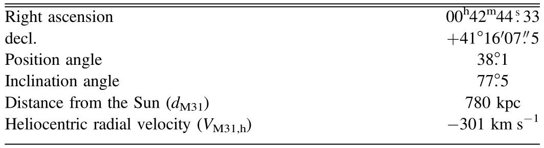
Table 1Basic Information of the M31 Galaxy

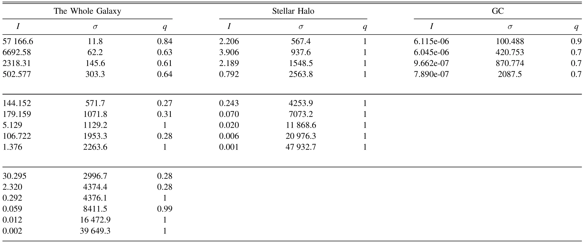
Table 2Parameters of MGE Fitting to the Three Populations Density

2.1.Kinematic Data

M31 is so close to us that the bright point sources in its field are resolved,like supergiants,PNe,and GCs,the LOS velocity of every single source is then obtained by spectroscopic data.We use a discrete data set composed of 48 supergiants,721 PNe,and 556 GCs with LOS velocity measured.They are mainly located at the inner 30 kpc and trace disk kinematics.In addition,we also include the LOS velocity dispersion of the accumulated halo stars at some discrete fields extending to～150 kpc.The spatial distribution of all the kinematic data is shown in Figure.1.The data points are aligned with the major axis of M31?s diskx′,and the zero-point is the galaxy’s center.

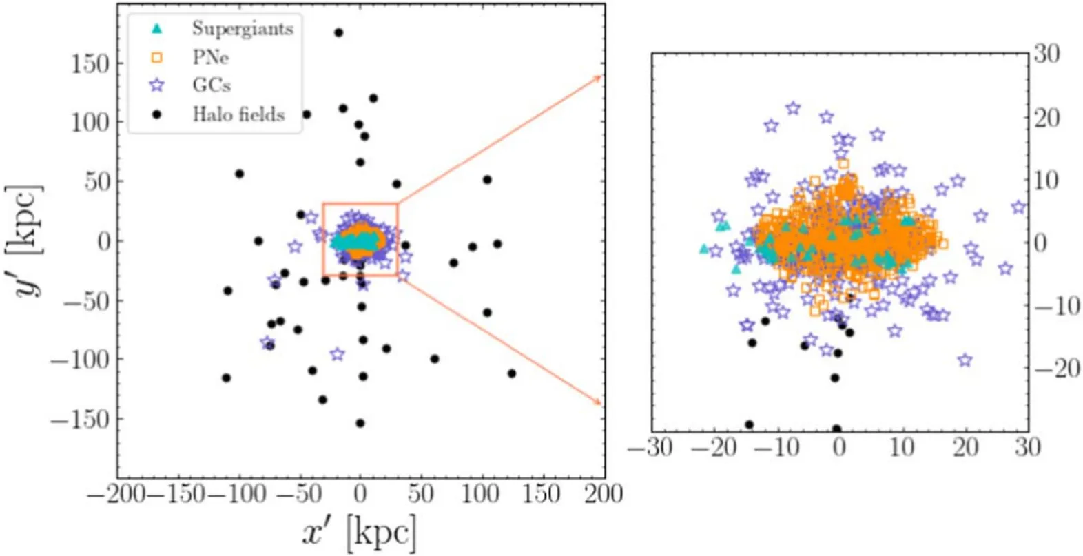
Figure 1.Position of the kinematic tracers.Orange squares,cyan triangles,and purple asterisks are discrete supergiants,PNe,and GCs.The black dots represent the positions with LOS velocity dispersion of accumulated halo stars measured.The discrete data points are primarily located in the inner ～30 kpc and mainly on the disk,while the velocity dispersion of accumulated halo stars extends to ～150 kpc.

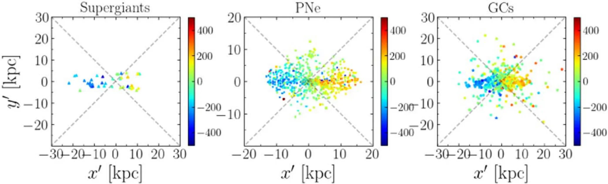
Figure 2.The line-of-sight velocity of discrete supergiants,PNe,and GCs.Each dot represents one object color-coded by its LOS velocity.Most of the tracers are located on the disk with a strong rotation.

The 48 supergiants we observed by LAMOST(see details in Liu et al.2022),with low-resolution spectra (LRS,R～1800).The typical error of LOS velocity is 10 km s?1.As shown in Figures1and2,the supergiants are located on the disk of M31 with strong rotation.

The catalog of PNe is from Halliday et al.(2006),Merrett et al.(2006) with the LOS velocities measured by the William Herschel Telescope,with a typical error of 6 km s?1.After carefully removing the contamination,they result in a clean catalog of 721 PNe in the disk and bulge of M31.As shown in Figure2,the kinematics of PNe generally follow the kinematics of the disk.Because PNe are remnants of stellar evolution,PNe and supergiants are supposed to have similar spatial and kinematical properties.We consider PNe and the supergiants together in the disk as one single population.

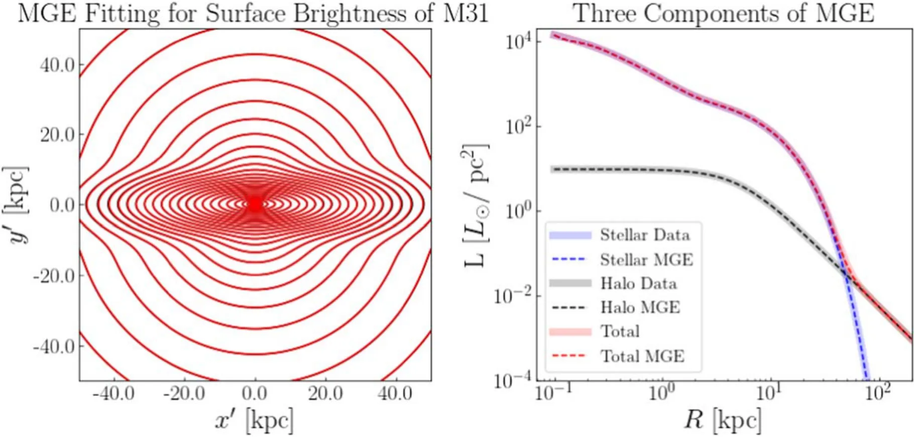
Figure 3.MGE fitting to the surface brightness of M31.Left: The 2D surface brightness of M31 (black) and the corresponding MGE fitting (red).Right: Surface brightness along the major axis x′.The total surface brightness of M31 (red solid curve) is a combination of the central galaxy (blue solid curve),which contains a sérsic bulge,an exponential disk,and a power-law halo(black solid curve)(Courteau et al.2011).The red,blue,and black dashed curves represent the corresponding MGE fitting.

The Revised Bologna Catalog of M31 GCs (RBC) presents all the confirmed GCs in M31 (Galleti et al.2004,2006,2007,2009),with a total number of over 600,and 554 of them have measured LOS velocities.This catalog is based on observations made at the 4.2 m William Herschel Telescope(WHT),the 3.5 m Telescopio Nazionale Galileo (TNG),and the Cassini 1.52 m telescope.Most GCs follow the rotation of the disk,while ～20% of them are located in the halo.GCs could generally have different origins compared to the stars.We thus consider GC a different population with the freedom to have different spatial distributions and kinematic properties from the stars.

The velocity maps of the supergiants,PNe,and GCs are shown in Figure2,each point is color-coded by its LOS velocity.The systematic velocity ofvsys=?301 km s?1of M31 has been subtracted.Almost all points are located with 30 kpc.Most of them are on the disk and follow the strong rotation,while there is a small fraction of PNe and GCs in the bulge regions and some in the halo.

The halo of M31 spans an area of ～15 deg2on the skyplane,with many substructures.Fifty discrete fields with over 5000 stars in the halo are observed through the Spectroscopic and Photometric Landscape of Andromeda’s Stellar Halo(SPLASH) Survey,which targets all four quadrants of stellar halo from M31?s center (Gilbert et al.2014,2018).After carefully modeling the contribution of substructures and smooth halo,the velocity dispersion profile of the smooth halo extending to ～150 kpc is provided (Gilbert et al.2018).As shown in Figure1,the halo fields cover a wide radial range from 9 ?R?175 kpc.In our model,halo stars will be considered a third population of kinematic tracers.

2.2.Photometric Data

We use a model of surface brightness fitting theI-band image of M31 out to 200 kpc(Courteau et al.2011).The model contains a sérsic bulge,an exponential disk,and a powerlaw halo.

The following sérsic function describes the surface brightness of the bulge component:

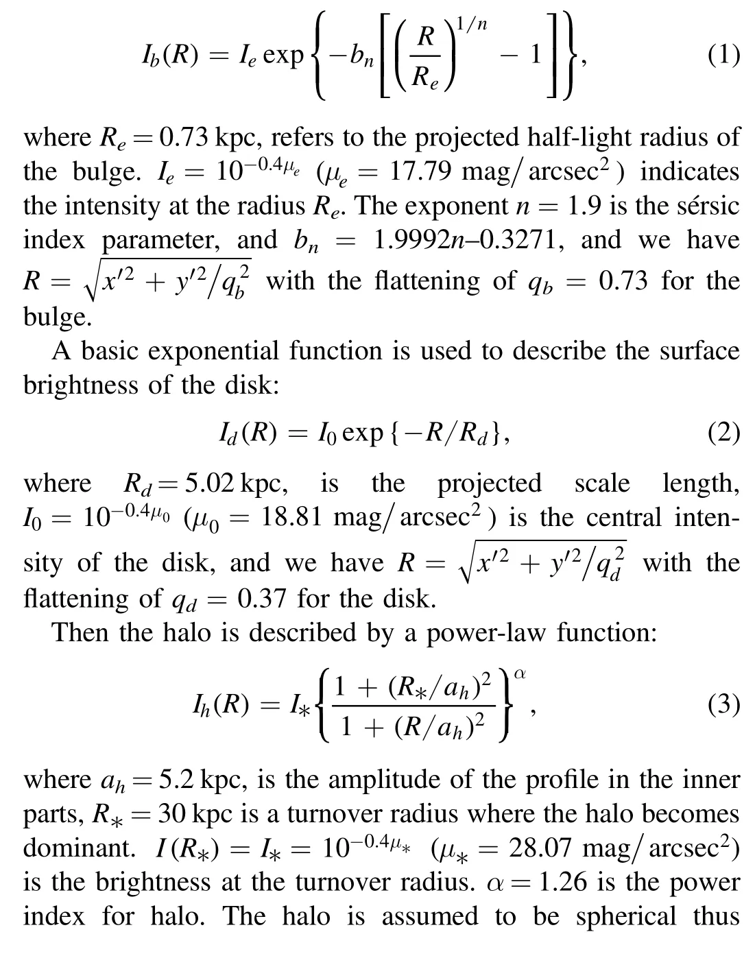
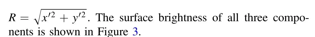
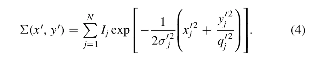
We require the surface brightness in the form of a Multi-Gaussian Expansion (MGE,Cappellari2002).MGE technique can fit a profile by a combination of several Gaussian components:

We first fit the total surface brightness of M31,which results in 15 Gaussian components.We use MGE of the whole galaxy to construct the model of stellar mass distribution to the gravitational potential,and for constructing the surface density profile of the tracer population with supergiants+PNe.Then,we fit the halo separately,which results in nine Gaussian components,which will be used to construct the surface density of the smooth halo.The MGE fitting is shown in Figure3,and the parameters are listed in Table2.

GCs have different spatial distribution compared to the stellar surface brightness.We construct the number density of GCs by counting all the confirmed 625 GCs,including the objects without LOS velocity measured.The MGE fitting to the surface number density of GC results in 4 Gaussian components.The surface number density and corresponding MGE fitting are shown in Figure4.The MGE parameters are listed in Table2,and they will be used as input for the surface density distribution of the tracer population using GCs.

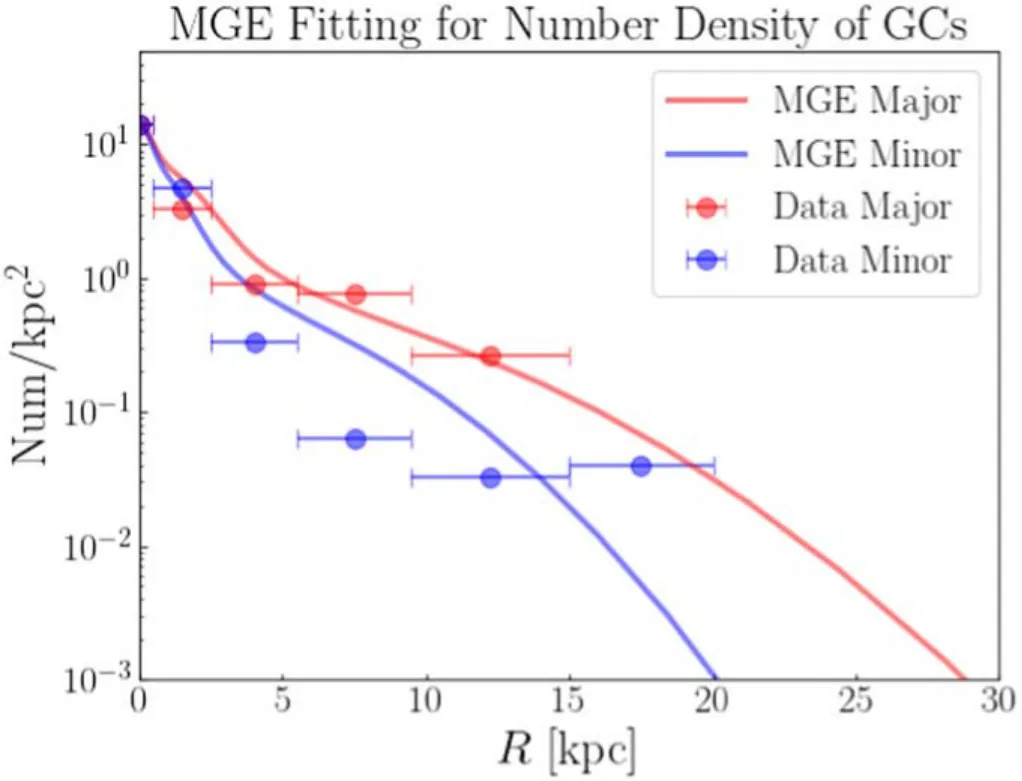
Figure 4.MGE fitting to the surface number density of GCs in M31.Red(blue)dots indicated the number counts in the bins along the major(minor)axis and the corresponding MGE fitting (red and blue solid curves).

3.Dynamical Models

We build a multiple-population discrete Jeans-Anisotropic-MGE (JAM) model to fit the three populations of kinematic tracers simultaneously.The three populations are organized in the same gravitational potential,while each population has its spatial distribution,rotation,and velocity anisotropy parameters in the JAM model.

3.1.Gravitational Potential

We construct the gravitational potential with stellar mass and DM mass.We have fitted an MGE model to the surface brightness of M31 at theIband,including the contribution of the bulge,disk,and halo.By assuming axisymmetric and taking an inclination angle of 77°.5,we deproject the 2D MGE surface brightness to obtain the 3D luminosity distribution of M31.Then by multiplying a stellar mass-to-light ratio(?I),we can obtain the stellar mass distribution of the galaxy.

We use a spherical generalized NFW(gNFW,Navarro et al.1996) halo for the DM distribution:

where ρsis the scale density,andrsis the scale radius of DM halo.Our data do not have strong constraints on the inner and outer slopes.We fix the inner slope γ=0 for a cored model and γ=1 for a cusped model,while the outer slope is fixed to be η=1.We thus have three free parameters in the gravitational potential: the stellar mass-to-light ratio ?I,the DM scale density ρs,and DM scale radiusrs.

3.2.JAM Model

We use a JAM model (Cappellari2008) to describe the kinematics of each tracer population in the gravitational potential.For an axisymmetric system in a steady-state,the Jeans equations are derived from the collisionless Boltzmann equation in the cylindrical coordinates are:

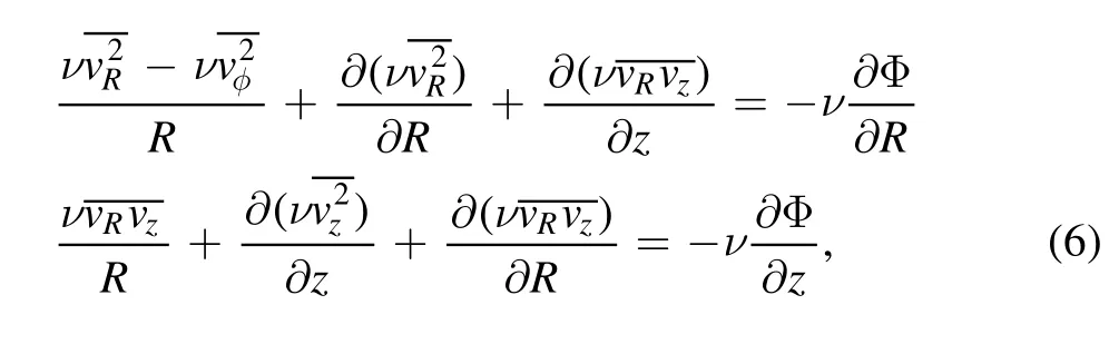
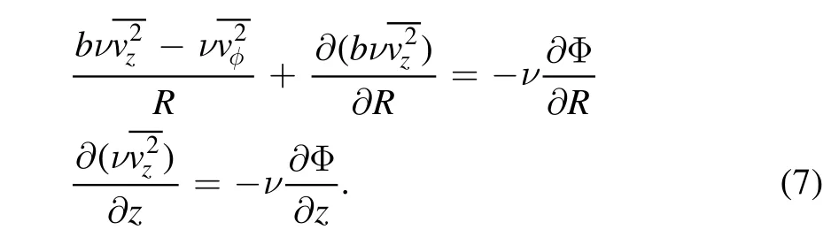
where Φ indicates the total potential of M31 that we try to recover,ν is the number density of each population.are the second velocity moments for tracers.In short,the left term of the Jeans equation is the dynamics information of each population,and the right term is the gravitational potential where tracers in the population are located.We have no information about those second velocity moments in these Jeans equations,making it impossible to have a unique solution.So we further give two assumptions that (1) the velocity ellipsoid is aligned with the cylindrical polar coordinate system,it means=0,and (2) the anisotropy parameter is a constant,assuming,in this case,the Jeans equations reduce to the following equations:

To calculate the first moments and compare them with the observational data (LOS velocity),we need to assume a rotation coefficient κ,which indicates the relative contributions of random and ordered motion.A rotation parameter κkcan be defined for each Gaussian componentkas follows:

In principle,a velocity anisotropy parameterband a rotation parameter κ can be set for each Gaussian component,resulting in a variation ofband κ as a function of radius.However,it will be too many free parameters that are hard to be constrained by the data in practice.We take constantband κ,thus only two free parameters for the internal kinematics of each tracer population.

Given the total gravitational potential,tracer number density,band κ,we can solve the full first and second moments describing the velocity distribution of an axisymmetric system at each position(R,z).Then we project the 3D model to the observational plane with an inclination angle,here for M31 known as 77°.5.By integrating along the LOS,we get the model predicted LOS velocity distribution(v,σ)at each position(x′,y′),which can be compared with observational data directly.

3.3.Maximum Likelihood Analysis

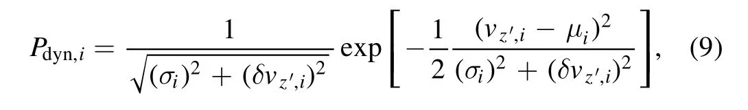
For a discrete data set withNpoints,each point at the position ofhas LOS velocityvz′,iwith error ofδvz′,i.The JAM model of each tracer population with given parameters will predict the LOS velocity distribution,a Gaussian distribution described by (μi,σi),at each positionin the observational plane.Then the probability of stariin a given model can be calculated by the following equation:

The probability of the whole data set withNpoints to be within the model is:

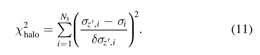
We have two populations of discrete tracer: (1) the stars at the bulge/disk regions traced by the combination of supergiants and PNe with a total number ofN1,(2)GCs also mainly distributed in the bulge/disk regions with a total number ofN2.We have the third population,the halo stars,with velocity dispersion measured from the accumulated halo stars atN3fields.For each point atwe have the LOS velocity dispersionσz′,iwith a error ofδσz′,i.We directly compare with the (σi) predicted by the model for the halo population,which results in:

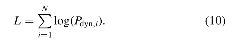
The minimum of χ2for accumulated halo stars and the maximum of the log-likelihood for the discrete supergiants+PNe and GCs can be determined at the same time by maximizing the combined likelihood defined as:

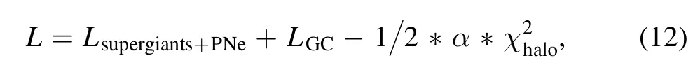
where α is the weight of different populations to the total likelihood,it is tuned to balance the fitting of different kinds of data.Here we fix α=2,which leads to a reasonably good fit for both the discrete data and the velocity dispersion profile of the halo.

3.4.Free Parameters

This section summarizes all the free parameters in the multiple-population JAM model of M31.The gravitational potential is a combination of stellar mass and DM halo.For the stellar mass,we have one free parameter:

(1) ?I,I-band stellar mass-light ratio;

The DM halo is a gNFW model with inner slope γ=1 for a cusped model or γ=0 for a cored model,and outer slope η=1 fixed,there are two free parameters left:

(2) ρs,dark matter scale density;

(3)ds,a combination parameter of ρsandrs,reducing the strong degeneracy between these two parameters,

For each tracer population,we have the freedom in the JAM model to determine its internal dynamics.For the stellar population in the central galaxy,traced by a combination of supergiants and PNe,we have two free parameters:

(4)λ1=-l n (1-β1),velocity anisotropy parameter of the stellar population,where β=1/(1?b)withbderived from the assumption ofas described in the JAM model,assuming thatbis the same for all Gaussian components,then λ is a constant along radius for this tracer population;

(5) κ1,the rotation parameter of the stellar population,indicating the relative contributions of random and ordered motion as defined in Equation (8).We assume the same κ for all Gaussian components,thus a constant κ along radius for this tracer population;

Correspondingly,there are two parameters for GCs population:

(6) λ2,velocity anisotropy of GCs population;

(7) κ2,rotation parameter of GCs population;

For the halo stars,we assume that it has zero rotation;thus only one free parameter is left:

(8) λ3,velocity anisotropy of the stellar halo.

4.Results

4.1.The MCMC Process

We run two sets of models: one with cusped DM halo(γ=1)and one with cored DM halo(γ=0).Here we illustrate the parameter exploration with the cusped model,similar figures for the cored model are included in theAppendix(FigureA1and FigureA2).We apply a Markov Chain Monte Carlo (MCMC) analysis to explore the parameter space using the EMCEE package developed by Foreman-Mackey et al.(2013).With eight free parameters,we run 200 steps,each step with 100 walkers.Figure5shows the evolution of the MCMC chain for the cusped model.The model quickly approached the best fit with ～100 steps,then gradually converged.The parameters keep constant,and the model likelihood does not change significantly in the last 100 steps.We take the last 50 steps as the post-burn chain and calculate the best-fitting parameters.In Figure6,we show distribution of the parameters in the post-burn phase.For most parameters,they are normally distributed as a Gaussian,with a higher likelihood in the central values.There is no noticeable degeneracy between the three tracer populations’kinematics parameters and the gravitational potential.However,the three parameters regarding the gravitational potential are degenerate,stellar mass distribution has degenerated with the DM mass distribution,and there is strong degeneracy between the two parameters,scale density and scale radius,describing the DM distribution.

4.2.Best-fitting Model

We calculated the probability of discrete data points in maximizing the model likelihood without binning.Only after evaluating model parameters then we bin both the data and model to show how well they match quantitatively.Figure7indicates a comparison between the observational data and the best-fitting models for supergiants+PNe and GCs.Figure8compares that to the velocity dispersion profile of the smooth halo.

In Figure7,the top row is the LOS velocity (left panel)and velocity dispersion (right panel) of supergiants+PNe.The bottom row shows the same for GCs.In addition,the data and model predictions were binned along the major and minor axes by using the cone-like divisions as shown in Figure2.We include 300 points in each bin,without overlapping between bins.For the observational data,the LOS velocity for each bin is the mean velocity of tracers in this bin,while the velocity dispersion is the standard deviation.The models are binned in the same scheme,but calculate the mean of velocity and velocity dispersion predicted at each position.The average of all the models with the 1σ confidence level is taken.The scatter of models within the 1σ confidence level is small thus we do not show.Our best-fitting models match well the observational data in both the LOS velocity and velocity dispersion,for both the supergiants+PNe and GCs populations.The cored and cusped models fit the data equally well,they are almost identical in Figure7.

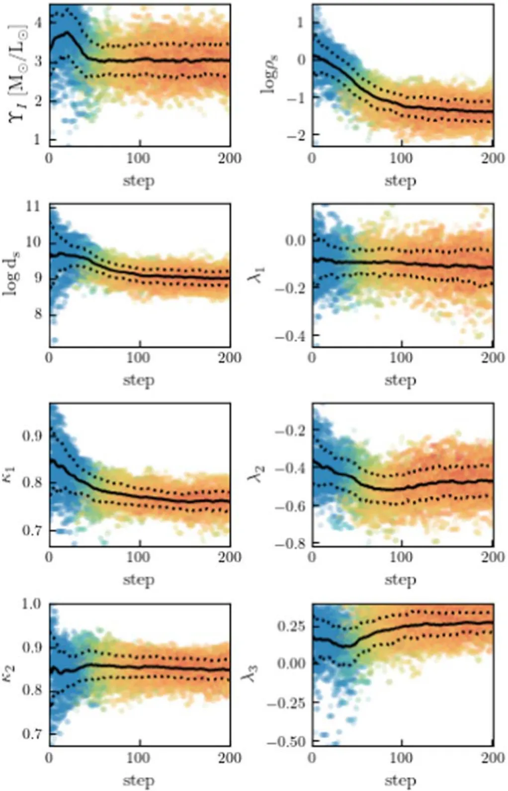
Figure 5.The evolution of MCMC chain in free parameter space for the cusped model.The points show the values sampled by 100 walkers at 200 steps,with color indicating the likelihood value from blue(low)to red(high).The first panel indicates the stellar mass-light ratio in I-band,then two parameters of DM halo ρs andds = in logarithm,then velocity anisotropy λ1 and rotation parameter κ1 of the stellar population,the corresponding parameters λ2 and κ2 for GCs population,λ3 for halo stars as we fixed the rotation parameter κ3 of 0.The solid line represents the average value of walkers at each step,and the dashed line represents the one sigma dispersion at each step.Dynamical modeling quickly approached the best fit with ～100 steps,then gradually converged.

In Figure8,we show the velocity dispersion profile of the smooth halo,and the comparison between the data and model.Our model matches well the velocity dispersion of halo stars atr?100 kpc.The dispersion from our model seems to be smaller than the data atr>100 kpc,but there are only two data points with large uncertainties.The discrepancy between data and model is not statistically significant.Again the cored and cusped models fit the data equally well,with velocity dispersion predicted by the best-fitting of the cusped model slightly larger than that from the cored model,but both are consistent with the data within 1σ error.

4.3.Mass Profile of M31

We show the enclosed mass profile of M31 obtained from our best-fitting models in Figure9.The total enclosed mass as a function of radius is shown in the top panel.The DM fraction as a function of radius is shown at the bottom.For both two models,the DM mass fraction reaches 50%at 5 kpc,it increases sharply atr?10 kpc,then increases slowly and reaches 90% at the end.

For the cusped model (γ=1,η=1): we obtained a stellar mass-to-light ratio of(M/L)I=3.0M⊙/L⊙,which corresponds to a total stellar mass ofM*=1±0.1×1011M⊙.Our best-fitting models preferrs=7.8±2.2 kpc,ρs=0.06±0.03M⊙/pc3for the DM halo,which corresponds toM200=7.0±0.9×1011M⊙,r200=184±8 kpc,and concentrationc=20±4.

For the cored model(γ=0,η=1),we obtained a stellar massto-light ratio of (M/L)I=2.7M⊙/L⊙,which corresponds to a total stellar mass ofM*=0.9±0.1×1011M⊙.Our best-fitting models preferrs=2.56±0.22 kpc,ρs=0.92±0.23M⊙/pc3for the DM halo,which corresponds toM200=5.1±0.4×1011M⊙,r200=165±5 kpc,and concentrationc=61±7.

In the central regions,our results are generally consistent with the results from the dynamical modeling constrained by IFU data(Bla?a Díaz et al.2018),they present a stellar mass of～7.5×1010M⊙within 15 kpc,while we have a stellar mass of 7.2±1.0×1010M⊙a(bǔ)nd 6.8±0.4×1010M⊙within 15 kpc for the cusped and core model,respectively.

The total enclosed mass profiles from the cusped and cored models are generally consistent with each other within the regions having the most observation data points(atr?30 kpc).While at the outer regions with weaker data constraints,the mass from the cored model is about ～15% lower than the cusped model.We reach a solution with a very high concentration for the cored DM halo model withc～60,thus the DM fraction of the cored model is slightly higher than that from the cusped model in the inner regions atr?30 kpc,with a lower concentration ofc～20 for the cusped model.

The DM inner slope γ is hard to constrain for galaxies like M31 because:(1)stellar mass is dominating in the inner few kpc,DM is only a small fraction,and (2) there is strong degeneracy between γ and the DM concentration.In our case,there is no preference for either of the models from the data fitting,the cusped and cored model fit the current data equally well.Cosmological simulations (Dutton &Macciò2014) reveal a correlation betweenM200and concentrationc,which is roughly consistent with observational results from lensing (Shan et al.2017).For a halo mass ofM200～6×1011M⊙,a concentration ofc～10 with 1σ scatter of ～5 is expected from the cosmological simulation.The cusped model withc=20±4 we obtained is consistent with the cosmological prediction within the 2σ scatter,while the cored model withc=61±7 has a too high concentration.In this sense,the cusped model is preferred over the cored model.

In Figure9,we compare our enclose total mass profile (red)with the previous results obtained from different dynamical methods using different tracers.We sorted the results in the literature into five categories according to the dynamical methods used and they are colored differently in the figure: (1) rotation curve based mass estimation(dark blue),(2)virial theorem based mass estimation(green),(3)DF-based dynamical model(orange),(4)tidal orbit modeling(gray),and(5)escape velocity based mass estimation(cyan).Different dynamical tracers,including H I,GC,PN,satellites,and streams are used.

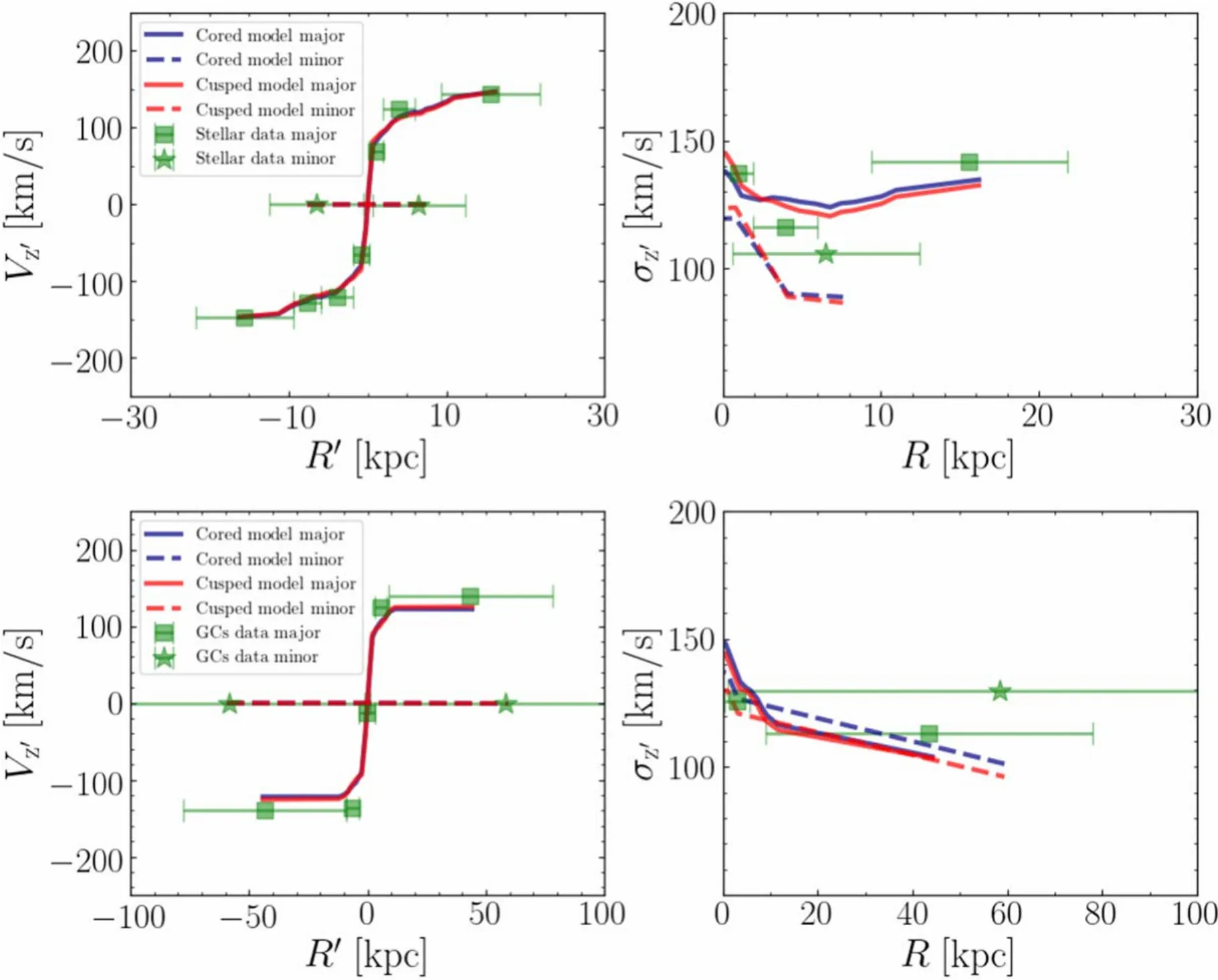
Figure 7.Comparison between the data and the best-fitting models for the two populations of discrete tracers.Top:Mean velocity(left)and velocity dispersion profile(right)for the stellar population in the bulge/disk regions.Dots with errorbar are the binned observational data,=blue curves are best-fitting of the cored model,and red are the cusped model.We have binned both the data and model along the major and minor axes by using the cone-like divisions as shown in Figure 2.The cored and cusped models match the data equally well.The red and blue curves are identical in the mean velocity profiles.Bottom:Similarly,for GCs,which are primarily located at r<30 kpc,with a few in the outer halo,cored models and cusped models also match GC’s mean velocity and velocity dispersion profiles.

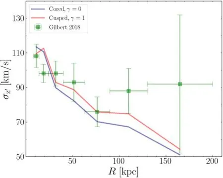
Figure 8.Comparison between data and model for the velocity dispersion profile of halo stars.Green dots are the velocity dispersion of accumulated halo stars as a function of radius (Gilbert et al. 2018).The blue and red curves are predicted from our best-fitting cored and cusped models,respectively.

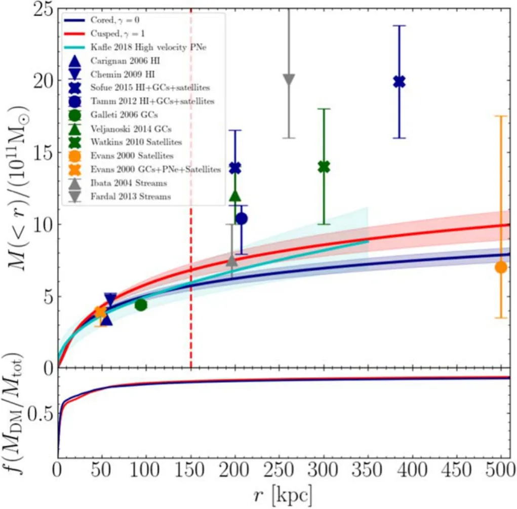
Figure 9.The enclosed mass profile from our best-fitting models and comparison with previous results.Top: The enclosed total mass profile.The blue curve is the result of our best-fitting cored model and red is the cusped model,with the shadowed regions indicating the 1σ uncertainty.Results from the literature are sorted into five categories according to the dynamical method they used: (1) rotation curve based mass estimation (blue),(2) virial theorem based mass estimation (green),(3) DF-based dynamical model (orange),(4)tidal orbit model(gray),and(5)escape velocity based mass estimation(cyan).The dynamical tracers used are labeled in the legend.The vertical dashed line indicates the radius where our kinematic data extended to.Our result is consistent with the lower side of allowed mass ranges in the literature.Bottom:DM fraction as a function of radius from our best-fitting model.DM fraction reaches 50%at 5 kpc,it increases quickly in the inner 10 kpc then slows down,and it finally reaches 90% for the whole galaxy.

In general,the total mass we obtained for M31 is at the lower side of the allowed ranges in the literature.Our result is consistent with the results obtained from the H I rotation curve (Carignan et al.2006;Chemin et al.2009),the DF-based dynamical model using different tracers (Evans et al.2000;Evans &Wilkinson2000),and that the high-speed PNe considering escape velocity of the potential Kafle et al.(2018),but much lower than the mass obtained in some other works,in particular,those using the kinematics of satellites (Watkins et al.2010),stellar streams(Ibata et al.2004;Fardal et al.2013)in the outer halo,and rotation curve mixed with H I,GCs and satellites (Tamm et al.2012;Sofue2015).

M31 is a complicated system with giant streams in the halo indicating a non-equilibrium state of the system(Ibata et al.2014;D’Souza&Bell2018).It suggests that M31 may have had a major merger at ～2 Gyr ago,which has heated the disk to be thicker but did not destroy it.Satellites and streams in the outer halo that are most likely to be accreted may not be well set down yet,thus they lead to over-estimation of the total mass.On the other hand,the tracers we used,stars,PNe and GCs,are mostly in the disk,well set down with regular kinematic properties,similarly to the H I rotation curve used in Carignan et al.(2006),Chemin et al.(2009)and PNe used in Kafle et al.(2018),thus they should trace the enclosed mass closely.But most of these tracers are located within the innerr?50 kpc of M31,thus having limited power to constrain the mass in outer regions.We also included the velocity dispersion profile of the smooth halo extending tor～150 kpc,which should help in constraining the mass profile.However,there are only two data points atr>100 kpc,and with large uncertainty,which are generally consistent with our current model within 1σ uncertainty.We need better data at the outer smooth halo for further understanding of the discrepancy of mass obtained from different methods and tracers.

5.Summary

We constructed a multiple-population discrete axisymmetric Jeans model for M31,combing three populations of kinematic tracers.The gravitational potential is a combination of stellar mass and DM mass represented by a spherical generalized NFW halo.We created two sets of models,one for a cusped DM halo with the inner slope γ=1,and one for a cored DM halo with γ=0.We included three populations of kinematic tracers organized in the same gravitational potential: (1) 48 supergiants combing 721 PNe are considered as the first population,which are mostly distributed in the disk,(2) 554 GCs are considered the second population,most of them are in the disk,and a small fraction is in the halo out to 30 kpc,(3) the stellar halo with velocity dispersion profile measured from accumulated halo stars is considered the third population.Each population is allowed to have its own spatial and kinematic properties in the multiple-population model.

Both the cusped and cored models fit the kinematics of all the three populations well,the cored model is not preferred due to a too high concentration ofc～60 obtained,which is much higher than predicted from cosmological simulations.With a cusped DM halo,we obtained a total stellar mass of 1±0.1×1011M⊙,DM halo virial mass ofM200=7.0±0.9×1011M⊙,and virial radius ofr200=184±4 kpc,with a concentration ofc=20±4.

The total mass of M31 we obtained is at the lower side of the allowed ranges in the literature.The discrepancy of mass obtained by different tracers in M31 may be partially caused by the non-equilibrium state of M31,which has had a recent major merger.Robust velocity dispersion profiles of the smooth halo atr?100 kpc are needed to improve the results.The uncertainties of the current LOS velocity dispersion profiles at the outer halo of M31 is about ～40 km s?1(Gilbert et al.2018),which is largely caused by the substructures with a systematic velocity of 10?100 km s?1.

M31 is at a distance of 780 kpc from us,with a proper motion of 0.01 mas/yr corresponding to 37 km s?1.Gaia DR3 has an uncertainty of ～0.01–0.02 mas/yr for the brightest stars atG<15(Gaia Collaboration et al.2021).The precision of future Gaia proper motion data is expected to be improved,indicating a factor of two reduction in the error for DR4 compared to DR3.CSST(the Chinese Space Station Telescope)is designed to have higher signalto-noise ratios at fainter magnitudes than Gaia.Thus future CSST proper motion measurements are promising to compensate for Gaia measurements at fainter magnitudes.If CSST can provide us with proper motion at such accuracy for some stars in the M31?s halo,it will help on removing the substructures thus reducing the uncertainty of velocity dispersion profiles of the smooth halo,and ultimately leading to a stronger constraint on its mass.

Acknowledgments

We acknowledge the science research grants from the China Manned Space Project with No.CMS-CSST-2021-B03.C.L.acknowledges the Grant with No.12033003.

Appendix

We show two figures on the MCMC results for the Cored model in the Appendix (FigureA1and FigureA2),similar to Figure5and Figure6for the cusped model shown in the paper.

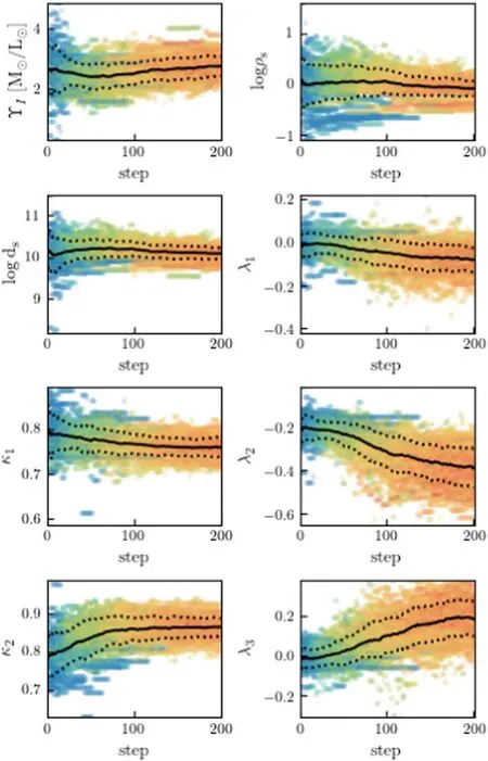
Figure A1.The evolution of MCMC chain in free parameter space in cored model.Similar to Figure 5.

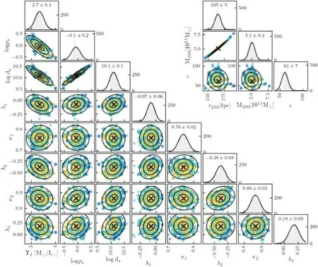
Figure A2.MCMC post-burn distribution in parameter space in cored model.Similar to Figure 6.