Yonghong LIU, Yongming XU, Yeping ZHANG, Xiuzhen HAN*, Fuzhong WENG, Chunyi XUAN, and Wenjun SHU

1 CMA Earth System Modeling and Prediction Centre, China Meteorological Administration (CMA), Beijing 100081

2 State Key Laboratory of Severe Weather, Chinese Academy of Meteorological Sciences, China Meteorological Administration, Beijing 100081

3 School of Remote Sensing and Geomatics Engineering, Nanjing University of Information Science & Technology, Nanjing 210044

4 National Satellite Meteorological Centre, China Meteorological Administration, Beijing 100081

5 Beijing Municipal Climate Centre, Beijing Meteorological Service, Beijing 100089

ABSTRACT

Key words: surface urban heat island, canopy urban heat island, vegetation coverage, albedo, sky view factor,

1. Introduction

In recent years, within the context of increasing global temperature and rapid urbanization, the climatic conditions of typical cities have been identified as one of the factors with the greatest influence on urban ecological environments. The most typical characteristic of urban climate is the urban heat island (UHI) effect. The UHI has become one of the most serious ecological problems of the 21st century (Voogt, 2002; Rizwan et al., 2008;Santamouris et al., 2015; Zhou et al., 2016). UHIs are generally categorized into canopy, boundary layer, underground, and surface UHIs (Oke et al., 2021). The canopy UHI (CUHI) and land surface UHI (SUHI) are currently two of the most extensively studied UHI types.CUHIs are generally measured at fixed near-surface meteorological stations or by mobile meteorological sensors,while SUHIs are primarily determined by using satellite remote sensing imagery. The rapid development and wide application of satellite remote sensing technology have made SUHIs a key reference metric for the assessment of urban thermal environments and for urban planning and construction (de Lucena et al., 2013; Liu et al.,2020a).

Many researchers have extensively investigated the SUHI as a metric for monitoring UHIs, focusing on its indicator value and the mechanisms underlying SUHI formation. SUHIs generally have clear spatial and temporal characteristics (van Hove et al., 2015). Their size and morphology are affected not only by the SUHI estimation methods used (Schwarz et al., 2011; Martin et al., 2015) but also by numerous other factors, such as climate types and weather conditions (Cheval et al., 2009;Du et al., 2016), phenology (Walawender et al., 2014),topography (Bokwa et al., 2015), types of land use (He et al., 2007), vegetation coverage and impermeable surface coverage (Imhoff et al., 2010; Connors et al., 2013), albedo (Peng et al., 2012), urban spatial morphology(Scarano and Sobrino, 2015; Yin et al., 2018), and anthropogenic heat (Wang et al., 2017). Given these factors and their different development characteristics, cities may each have unique SUHI distribution patterns (Oke et al., 2021). Therefore, studying the causes of SUHIs in a city requires the consideration of as many characteristic factors related to the city’s spatial structure as possible in addition to its climatic and geographical background conditions. Moreover, subsequent identification of the primary factors affecting the SUHI is essential to provide a reference and basis for urban planning and UHI control.

The SUHI displays a more distinct spatial pattern,while the CUHI is more temporally consistent. Therefore, studying the SUHI and CUHI in tandem can yield a better understanding of the spatial and temporal variation in a city’s thermal environment (Schwarz et al.,2012; Mohan et al., 2013). From early on, researchers noticed a marked difference (Oke and Cleugh, 1987;Roth et al., 1989) and a lack of a simple correspondence between the SUHI and CUHI (Arnfield, 2003). The difference in temperatures and peak times of the SUHI and CUHI depend on urban and rural surface properties [e.g.,humidity, aerodynamic roughness, albedo (AB), emissivity, thermal admittance, and seasonal, geographical, and climatic conditions] (Voogt and Oke, 2003). Generally,the CUHI and SUHI peak at night and during daytime,respectively, and the SUHI is often higher than the CUHI and undergoes the greatest spatial changes during the daytime, while the most considerable spatial variation in the CUHI may occur at night (Schwarz et al., 2012; Sun et al., 2015). The SUHI usually peaks in the early afternoon and differs from the CUHI by up to 9–10°C. The CUHI is inconspicuous during the daytime and only displays the same pattern as that of the SUHI after sunset and at night (Anniballe et al., 2014; Zhang et al., 2014).A study examining the summer UHI in Birmingham of the British city found the following (Azevedo et al.,2016): (1) the SUHI is higher than the CUHI both during daytime and at night; (2) the SUHI is more related to land use, while the CUHI is more closely related to the direction of atmospheric advection; and (3) both the SUHI and CUHI increase as the stability of the atmosphere increases at night. Another study investigating the SUHI in Hong Kong showed that the spatial geometric features [e.g., building density (BD), the standard deviation of building heights (BSD), and sky view factor(SVF)] of a city affect its daytime and nighttime SUHI to considerably different extents (Yang et al., 2021). From a surface energy balance perspective, Zhou et al. (2018)analyzed the main cause of the difference between daytime and nighttime SUHIs. They noted that a daytime SUHI is caused predominantly by the reflection of solar radiation by the surface and the decrease in the latent heat flux at the surface. In contrast, a nighttime SUHI results mainly from the slow release of the large amount of heat absorbed by the surface during the day. These formation mechanisms differ considerably from those of daytime and nighttime CUHIs (Oke et al., 2021).

To date, researchers have examined the relationship between the formation mechanism of SUHIs and CUHIs in Beijing. The SUHI and CUHI metrics for Beijing show consistent interannual trends (Liu et al., 2014).However, in terms of their values and spatial distribution patterns, these two metrics differ notably during the daytime but are consistent at night (Sun et al., 2015; Liu et al., 2016). In terms of the formation mechanism of the UHI, the impervious coverage (IC) can explain 49%–54% of the variation in the nighttime CUHI and 31%–38% of the variation in the daytime SUHI (Wang et al.,2017), while the vegetation coverage (VC) and floor area ratio (FAR) can explain over 90% of the variation in the daily maximum land-surface temperature (LST) in Beijing (Zhao et al., 2011). Liu et al. (2021a) studied the effects of eight spatial pattern metrics and three land-surface metrics on the CUHI. They found that the urban spatial pattern metrics surpassed the land-surface metrics(i.e., VC, IC, and AB) and became important drivers of the variation in the CUHI and that these metrics could explain 46.8%–79.6% of its variation. However, whether these metrics similarly affect the SUHI and the mechanism by which they affect the difference between the SUHI and CUHI currently remain elusive.

Many published studies examining the effects of urban spatial landscape (USL) metrics on the SUHI and CUHI are case studies based on short-term (mostly summer)metrological or satellite observations (Zhao et al., 2011;Tsoka et al., 2017; Yang et al., 2021) or simulate the thermal environment by constructing an ideal parametric building form model (Touchaei and Wang, 2015; Jamei et al., 2017). Very few studies have investigated the long-term average impact of the actual USL on the CUHI in all weather conditions. This limitation can be ascribed to the following factors. Most published CUHI-based studies are performed based on data collected at meteorological stations. Limitations imposed by the density and construction time of meteorological stations present a challenge to the determination of a detailed spatial distribution pattern of the CUHI over a long period of time and therefore preclude a comparison with the distribution pattern of the SUHI at high spatial and temporal resolutions derived from satellite imagery. Moreover, obtaining fine USL pattern metrics at an urban scale is also a difficulty that limits comparisons of the impact of USL pattern metrics on the CUHI and SUHI.

To address the above problems and considering spatial and temporal representativeness, this study first produces a high-spatial-resolution estimate for the distribution pattern of the SUHI in Beijing based on a long time series of satellite data. The estimate is then compared with the fine spatial and temporal distribution patterns of the CUHI derived from a long time series of data collected at a high-density network of automatic meteorological stations (AMSs). In addition, considering that the SUHI is affected primarily by the geometrical, radiation,thermal, humidity, and aerodynamic properties of the surface, 11 USL pattern metrics—including those that can reflect the geometrical and thermal properties of a city [i.e., building height (BH), BD, fractal dimension(FD)], AB (a metric that reflects surface radiation properties), land-surface metrics that reflect the thermal and humidity properties of the surface (i.e., VC and IC), and roughness length (RL; a metric that reflects the aerodynamic properties of the surface)—are selected. VC mainly reduces air temperature and increases humidity through evapotranspiration, while IC mainly reduces humidity by reducing evaporation and increases air temperature by sensible heat for impervious surfaces. RL and FAI indirectly affect the urban land surface temperature mainly through wind speed and turbulence; for example,the high value of land surface temperature generally appears in flat topography and on leeward surfaces with weak turbulence, and the low value appears on the rough surface with wind (Oke et al., 2021). The spatial distribution of each of these 11 USL metrics is determined through remote sensing and geographic information system (GIS) technology in combination with morphological models. On this basis, the impact of these metrics on the SUHI and CUHI and their differences are investigated.Notably, the impact of these metrics on the CUHI has been studied in the relevant literature (Liu et al., 2021a).Based on the research results, this paper further studies the impact of the metrics on the SUHI and explores the difference in the influence of these metrics on the SUHI and CUHI. The results of this study can provide a reference and basis for selecting different urban planning metrics for CUHI and SUHI control.

2. Study area

Beijing is located in the northern part of the North China Plain and is surrounded by mountains to the west,north, and east (Fig. 1a). Its total area is 16,410 km2, approximately 38% of which is the plains area. The study area consisted of the parts of the plain with elevation ≤100 m in Beijing’s central urban area (CUA), which is approximately 1236.7 km2in area, with most blocks in the study area covered by urban built land and green spaces (Fig. 1b).

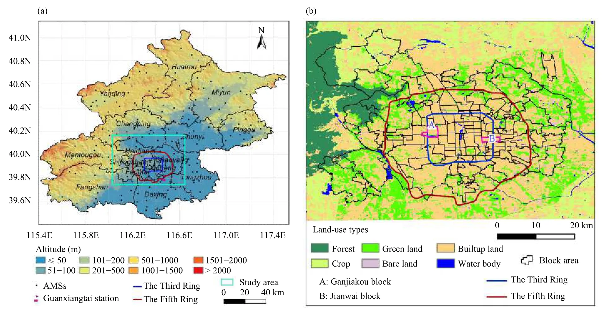
Fig. 1. (a) Topography and automatic meteorological observation stations (AMSs) in Beijing and (b) land-use types in the study area.

The study area lies in the warm temperate zone, and the K?ppen climate type is DWA (Wang et al., 2020).Summer (from June to August) is hot and rainy, and winter (from December to February) is cold and dry. The hottest month is July, with an average temperature of 26.7°C, and the coldest month is January, with an average temperature of ?3.1°C (Liu et al., 2021b). Beijing is a megacity with a permanent population of approximately 21.88 million at the end of 2021. The urbanization rate has reached 87.5%, and the built-up area is 1469 km2. The UHI in Beijing is considerable and is larger than that in Changchun, Wuhan, and Guangzhou at different latitudes in the same eastern monsoon region in China (Jia et al., 2021).

3. Methods and data

3.1 Calculation of CUHI and SUHI

Here, using an urban?rural dichotomy, CUHI and SUHI can be calculated as follows:where CUHI (°C) is the canopy urban heat island intensity, AT (°C) is the air temperature of the AMS in the study area, and ATr(°C) is the average temperature of the representative rural background stations. SUHI (°C)is the land surface urban heat island intensity, LST (°C)is the land surface temperature, and LSTr(°C) is the average land surface temperature of the representative rural background area.

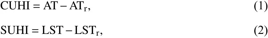
In this paper, taking the rural background of the UHI as the reference for remote sensing observations (Liu et al., 2021a) and using the altitude, land-cover type data,and annual mean nighttime light intensity (Fig. 2a) extracted from the Suomi National Polar-orbiting Partnership (Suomi-NPP) Visible Infrared Imaging Radiometer Suit (VIIRS) satellite data in 2018, which can be downloaded for free from NASA’s National Environmental Information Data Center, the rural background area and six representative rural stations were selected from the 197 AMSs in Beijing (Fig. 1a), as shown in Fig. 2b.

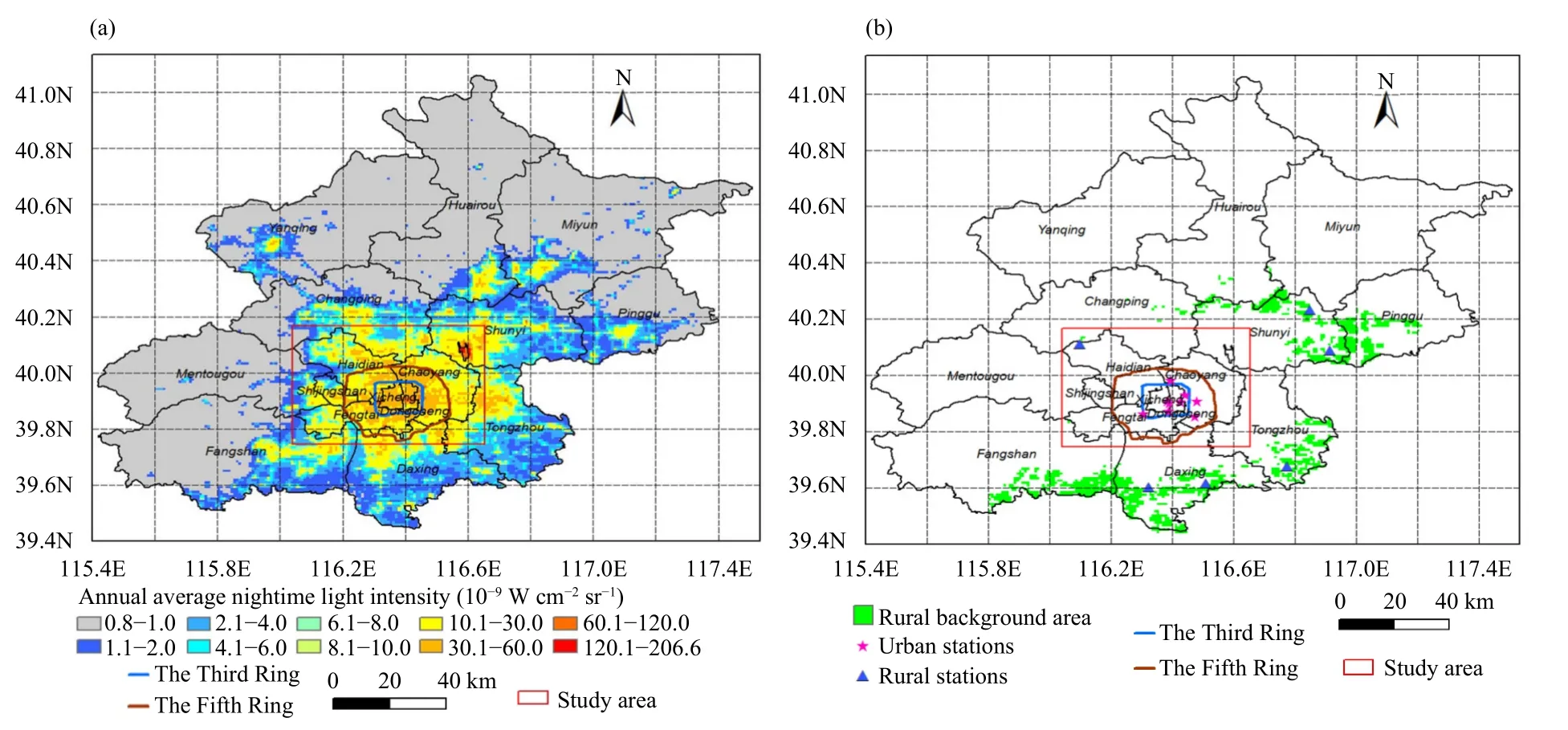
Fig. 2. (a) Annual mean nighttime light intensity in Beijing in 2018 extracted from NPP VIIRS satellite data and (b) distribution of the rural background areas and rural and urban stations in Beijing.

Hourly air temperature data for the period of 2009–2018 from 197 AMSs provided by the Beijing Meteorological Information Centre were used to calculate the mean CUHI values in different time periods and were spatially interpolated to generate the CUHI maps of Beijing’s CUA with a 1-km spatial resolution.

Moderate Resolution Imaging Spectroradiometer(MODIS)-Terra and MODIS-Aqua 8-day composite average LST products (MOD11A2 and MYD11A2) with a 1-km spatial resolution for Beijing during 2009–2018 were used to calculate the mean SUHI values in different time periods, which can be downloaded for free on the official website of NASA’s Land Processes Distributed Active Archive Center.

3.2 Calculation of USL metrics

Table 1 summarizes the meaning and calculation of methods for 11 USL metrics.

Based on the locations of buildings and information on floors on a 1 : 2000 topographic map of residential land and buildings of Beijing in 2017 provided by the Beijing Institute of Surveying and Mapping, BH was estimated under the assumption that each floor had a mean height of 3 m. In addition, GIS spatial analysis and image processing techniques were employed in combination with the calculation methods for relevant metrics in Table 1 to produce spatial distribution maps with 500-m spatial resolution for the BH, BD, FAR, BSD, RL, frontal area index (FAI), and SVF (Liu et al., 2021a).

The clear sky Landsat 8 Operational Land Imager(OLI) remote sensing image (row/path: 123/32) on 10 July 2017 in Beijing from the Open Spatial Data Sharing Project by the Institute of Remote Sensing and Digital Earth (RADI), Chinese Academy of Sciences, was used with the calculation methods described in Table 1 to estimate VC and IC maps (Liu et al., 2021b) and FD map(Liu et al., 2020b) with 500-m spatial resolution.

The albedo product MCD43A3 (v006 version) with MODIS 500-m resolution for Beijing in 2017, which can be downloaded for free from the official website of NASA’s Land Processes Distributed Active Archive Center, and the total radiation and scattered radiation data collected at the representative meteorological station Guanxiangtai (Fig. 1a) in Beijing in 2017 were used to produce annual and seasonal mean AB estimates for Beijing, as shown in Fig. 3. Low-AB (< 0.14) zones are distributed over a large portion of the CUA of Beijing,with pronounced low-AB values (< 0.10) occurring near the CBD (Central Business District) around the east Third Ring Road.

3.3 Spatial units (blocks)

Here, 115 spatial units (i.e., blocks in Fig. 1b) unaffected by topographic conditions in the CUA are analyzed to examine the difference between the impact of the USL metrics on the SUHI and CUHI. Analysis of the 3.93-km2Jianwai block (area A in Fig. 1b) and the 6.56-km2Ganjiakou block (area B in Fig. 1b) is presented as an example. Figure 4 shows the spatial distribution of the BH and SVF for each of the Jianwai and Ganjiakou blocks and the means of the USL metrics for these two blocks calculated by using the methods in Table 1.

Fig. 3. (a) Annual, (b) spring, summer, autumn, and winter mean AB values for the CUA in 2017.

Fig. 4. Spatial distribution patterns (resolution: 5 m) of the BH and SVF and means of the USL metrics (BH, BD, FAR, BSD, RL, FAI, SVF,FD, IC, VC, and annual AB) for the (a) Ganjiakou and (b) Jianwai blocks in Beijing.

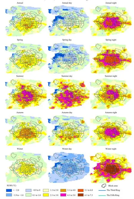
Fig. 5. Spatial distributions of the mean SUHI with 1-km spatial resolution for the 115 block areas in Beijing’s CUA during different periods of 2009–2018.

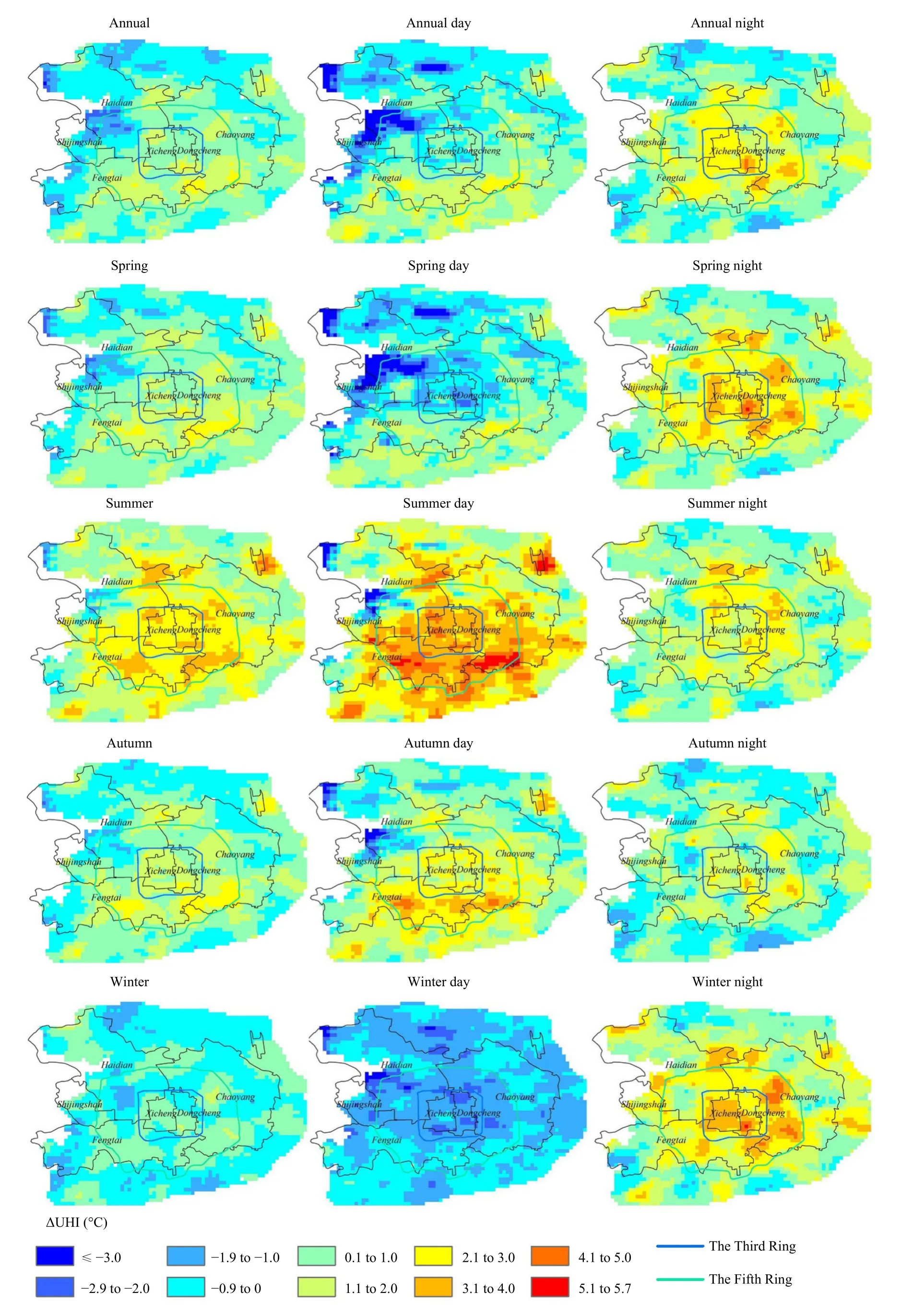
Fig. 6. Spatial distributions of ΔUHI with 1-km spatial resolution for Beijing’s CUA during different periods of 2009–2018.

The area of 115 spatial units and the average, minimum,maximum, and standard deviation of 11 USL metrics are shown in Table 2. Except for the seasonal changes in AB, other USL metrics are assumed to exhibit no seasonal change. Then, estimating the USL metrics and the SUHI and CUHI for the 115 block units allows an analysis of the difference between the impact of the USL metrics on the SUHI and CUHI.

Table 1. Meanings and calculation methods for the 11 USL metrics selected in this study

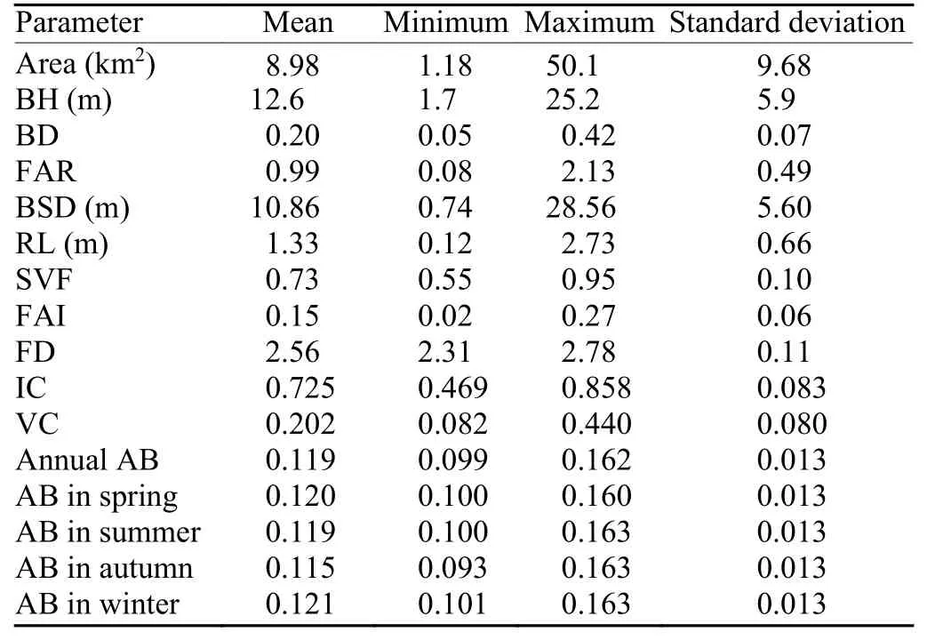
Table 2. Statistical information of 115 block spatial units in the study area

To compare the SUHI and CUHI, daytime and nighttime SUHI values are derived from MODIS-Aqua images taken at 1330 and 0130 LT (local time), respectively, while daytime and nighttime CUHI values are determined from spatially interpolated maps for 1400 and 0200 LT, respectively.

4. Results and analysis

4.1 Spatiotemporal distributions of SUHI and CUHI

Figures 5 and 6 show the spatial distribution patterns of the mean SUHI and the difference (ΔUHI) between the mean SUHI and the mean CUHI in the CUA in 15 time periods (i.e., annual, annual daytime, annual nighttime, spring, spring daytime, spring nighttime, summer,summer daytime, summer nighttime, autumn, autumn daytime, autumn nighttime, winter, winter daytime, and winter nighttime) over 2009–2018, respectively. Table 3 compares the mean SUHI and CUHI values within the Fifth Ring Road in the corresponding time periods. Ana-lysis of these data in combination with the spatial and temporal patterns of the CUHI (Liu et al., 2021a) reveals the following.

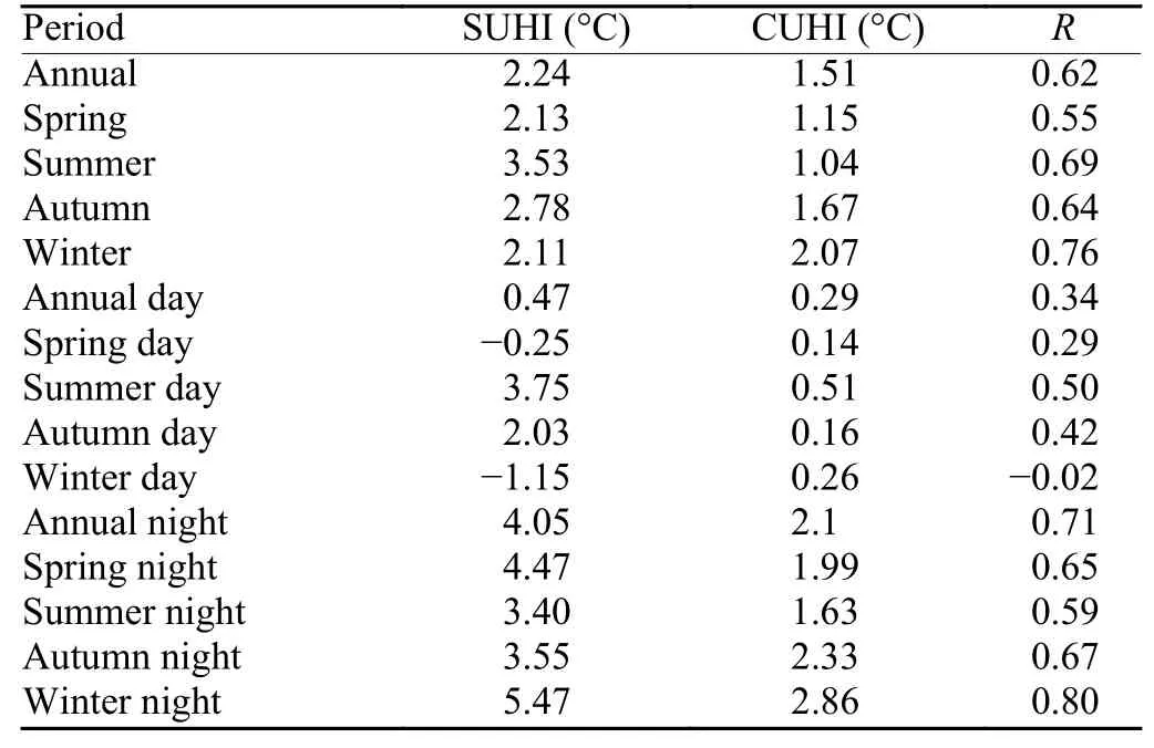
Table 3. Mean SUHI and CUHI within the Fifth Ring Road and R values for the correlation between the SUHI and CUHI in the 115 blocks in Beijing’s CUA during different periods of 2009–2018

Annual and nighttime SUHI values display similar fixed spatial distribution patterns. A similar finding is observed in the CUHI. However, the SUHI and CUHI differ notably in their spatial distribution patterns. Whereas the SUHI is primarily manifested in a single large pieshaped heat island, the CUHI mainly appears as four scattered heat island centers. While the spatial distribution pattern of the nighttime SUHI is consistent among seasons, the SUHI varies considerably among seasons.The SUHI is the highest (5.47°C) at night in winter,which is consistent with the time when the highest CUHI(2.86°C) occurs. The spatial distribution pattern of the SUHI during the daytime differs markedly from that at night. During the daytime, the SUHI mainly appears as a heat island in summer and autumn (with intensities of 3.75 and 2.03°C, respectively) and as a cold island in winter and spring (with intensities of ?1.15 and ?0.25°C,respectively). This finding differs from the consistent spatial distribution pattern of the CUHI during the four seasons and can be ascribed to the following factor. The seasonal variation in the SUHI depends largely on the variation in surface features, e.g., vegetation cover and particularly, soil humidity (Oke et al., 2021). The surface in the suburban area of Beijing is covered primarily with sparsely vegetated, dry, and bare soil in winter and spring and highly vegetated and moist soil in summer and autumn, while the surface of the urban area of Beijing is covered predominantly with concrete. At night,the dry surface in winter cools to a much greater extent than the moist surface in summer in the suburban area,while the decrease in the LST in the urban area varies nonsignificantly among seasons. Consequently, the SUHI is the highest on winter nights and lowest on summer nights, with the values on spring nights and autumn nights in between. Because the specific heat capacity of dry, bare soil is lower than that of concrete, bare soil warms up more quickly than concrete under direct sunlight. Therefore, during the daytime, the sparsely vegetated, dry, bare soil in the suburban area warms up considerably more quickly than the urban surface in winter and spring. Consequently, a cold island tends to occur during the daytime in winter and spring. In contrast, in summer and autumn, the soil in the suburban area is moist and has a dense vegetation cover that has a cooling effect through evapotranspiration. Therefore, the suburban surface warms up much more slowly than the urban surface. Hence, a heat island tends to occur during the daytime in summer and autumn.

Analysis of the seasonal means reveals that the SUHI is the highest (3.53°C) in summer and lowest (2.11°C) in winter. The opposite finding is observed for the CUHI:its highest (2.07°C) and lowest (1.04°C) values occur in winter and summer, respectively. Analysis of the daytime and nighttime variation shows the following. The annual nighttime mean values of the SUHI and CUHI are higher than their respective annual daytime mean values.From a seasonal perspective, the SUHI is higher at night than during the daytime in each season except summer,which differs from the finding for the CUHI, which is higher at night than during the daytime in all seasons. In addition, during the daytime in summer, the SUHI(3.75°C) is significantly higher than the CUHI (0.50°C).During the daytime in winter and spring, the CUHI shows no notable heat island effect (with intensity levels of ?0.02 and 0.29°C, respectively), whereas the SUHI displays a cold island effect over a large area with an intensity considerably lower than that of the CUHI. This phenomenon is particularly pronounced during the daytime in winter (the corresponding SUHI is ?1.15°C).

Notably, the maximum SUHI occurs at night in winter. This finding contradicts the generally established conclusion that the maximum SUHI usually occurs during the daytime in summer (Oke et al., 2021). However,this result is consistent with the derivation obtained by Wang et al. (2017) from MODIS data with farmland as the background, where the SUHI at night in winter(5.04°C at 0130 LT) is higher than that during the daytime in summer (4.49°C at 1330 LT) in Beijing. This finding may be largely attributed to the significant anthropogenic heat factor resulting in warmer winters in Beijing.

Analysis of the spatial distribution of ΔUHI (Fig. 6)reveals the following. There are similarities in the spatial distribution patterns of the nighttime ΔUHI across the four seasons, suggesting a high level of spatial consistency between the SUHI and CUHI at night. In contrast,the daytime spatial distribution patterns of ΔUHI differ significantly across the four seasons, indicating a very low level of consistency between the SUHI and CUHI during the daytime. The annual and seasonal nighttime mean ΔUHI values are mainly positive, suggesting that the SUHI is generally higher than the CUHI at night (as shown in Table 3). The daytime ΔUHI is mainly negative (up to below ?2°C) in winter and spring and positive(up to above 5°C) in summer and autumn, with its maximum value occurring in summer. During the daytime in summer, the mean SUHI and CUHI values within the Fifth Ring Road are 3.75 and 0.51°C, respectively. The above finding can be attributed to the following factors.Solar radiation is intense during the daytime in summer.The urban surface is composed primarily of concrete and therefore warms much more than the rural surface covered with densely vegetated, moist soil, resulting in a very high SUHI. The atmospheric temperature results from heating by longwave radiation from the surface.The atmosphere is highly volatile and turbulent under sunlight in summer, resulting in frequent heat exchange between the urban and rural areas, which in turn leads to a low CUHI.

Table 3 summarizes the values of Pearson’s correlation coefficient (R) for the spatial correlation between the mean SUHI and CUHI in the 115 blocks in Beijing’s CUA for different periods of 2009–2018. The spatial correlation between the SUHI and CUHI differs notably with the time period. The metricsRvaries between ?0.02 and 0.80, with an annual mean of 0.62. Analysis of the meanRvalues for the four seasons reveals that the correlation is the strongest in winter (R= 0.76), followed by that in summer (R= 0.69) and that in autumn (R= 0.64),and that the correlation is the weakest in spring (R=0.55). Analysis of theRvalues for the daytime and nighttime correlations shows that the spatial correlation is generally stronger at night than during daytime, with the annual nighttime meanR(0.71) being significantly higher than the annual daytime meanR(0.34). Of the four seasons, the correlation is the strongest (R= 0.80) at night in winter, followed by that at night in autumn (R= 0.67)and that at night in spring (R= 0.65), while the correlation at night in summer is the weakest (R= 0.59). The daytime correlation is generally weak in each season, and the strongest daytime correlation occurs in summer, with anRof only 0.50. This finding shows a high level of consistency between the SUHI and CUHI at night but a notable difference between them during daytime, which agrees with the analysis of the spatial distribution pattern of ΔUHI. Therefore, the SUHI can serve as an important indicator of the CUHI at night but is ineffective at indicating the CUHI during the daytime, which can be attributed mainly to the following factors. The daytime CUHI determined from meteorological observations depends on not only surface heat radiation under sunlight but also the atmospheric heat exchange caused by the volatility of the atmosphere under solar radiation and the anthropogenic heat released from the intense human activity during daytime. Consequently, the correlation between the daytime SUHI and CUHI is weak. At night, the atmosphere is stable, resulting in a considerable decrease in both the horizontal and vertical atmospheric heat exchange. Consequently, the temperature of the atmosphere depends primarily on surface heat radiation. Therefore, there is a high level of consistency between the SUHI and CUHI.

4.2 Correlations between USL metrics and SUHI/CUHI

Figures 7 and 8 show the spatial correlations between the mean SUHI and CUHI and various USL metrics (expressed asRvalues) for the 115 blocks during 15 time periods of 2009–2018 and the maximum spatial correlation coefficients (Rmax) for the 15 time periods, respectively.

(1) BH, BD, FAR, and BSD. Spatially, these four building form metrics are strongly positively correlated with both the SUHI and CUHI in most time periods (Fig.7). In other words, an increase in BH, BD, FAR, and BSD results in an increase in both the SUHI and CUHI.However, these correlations occur mostly at night, with absoluteRvalues generally above 0.5. In addition, these metrics are more strongly correlated with the SUHI than the CUHI. During the daytime, these four building form metrics are weakly correlated with the SUHI and CUHI,with absoluteRvalues generally below 0.4. In contrast to the CUHI, BH, FAR, and BSD are to some extent negatively correlated with the SUHI during the daytime in winter, withRvalues ranging from ?0.5 to ?0.4. Due to the generally weak correlations during the daytime, the strength of the annual and seasonal correlations between each metric and the SUHI and CUHI varies. For example, BD is more strongly correlated with the SUHI than with the CUHI in winter. However, an opposite pattern is found for their annual correlations. Analysis of the strongest spatial correlations (Fig. 8) reveals the following. The FAR is correlated with the SUHI and CUHI to similar extents (Rmax= 0.75) that are greater than those to which the other three metrics are correlated with the SUHI and CUHI. This phenomenon occurs because the FAR combines the impact of BH and BD on the thermal environment and therefore has a substantial maximum impact on the SUHI and CUHI. The maximum correlations of BH, BD, and BSD with the SUHI (Rmax= 0.68,0.71, and 0.64, respectively) are stronger than their maximum correlations with the CUHI, suggesting that these three metrics may have a higher maximum impact on the SUHI than on the CUHI.

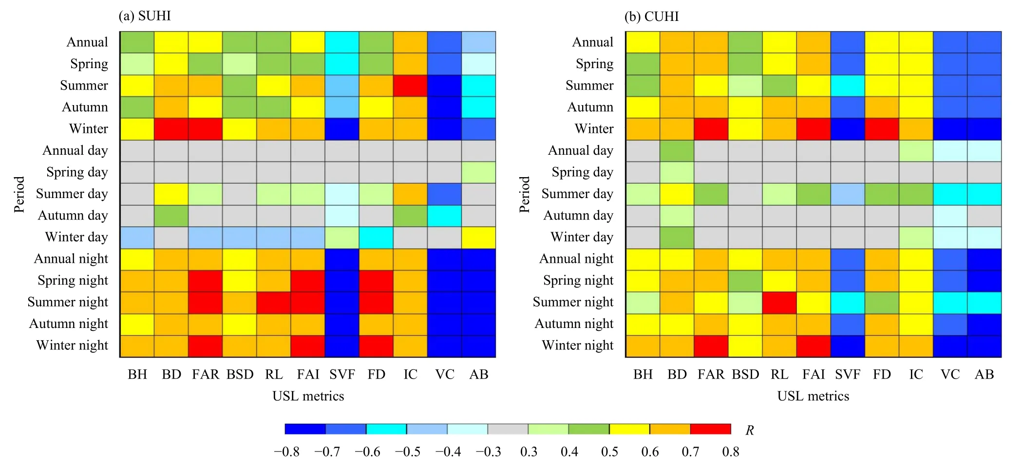
Fig. 7. Distributions of R of the (a) SUHI and (b) CUHI and the USL metrics (i.e., BH, BD, FAR, BSD, RL, FAI, SVF, FD, IC, VC, and AB)for Beijing’s CUA during different periods of 2009–2018.

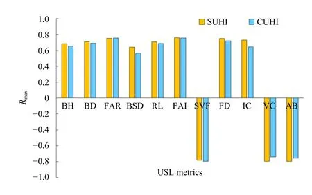
Fig. 8. Comparison of Rmax of the SUHI and CUHI with each USL metric (i.e., BH, BD, FAR, BSD, RL, FAI, SVF, FD, IC, VC, and AB)for Beijing’s CUA during different periods of 2009–2018.

(2) RL, FAI, and FD. Spatially, RL, FAI, and FD are all significantly positively correlated with the SUHI and CUHI in most time periods, particularly at night, withRvalues generally above 0.60. However, during the daytime in winter, these three parameters are strongly negatively correlated with the SUHI, withRvalues ranging from ?0.6 to ?0.4. This type of strong negative correlation is not observed in the CUHI. In terms of the maximum spatial correlations, theRmaxvalues for the correlations of RL, FAI, and FD with the SUHI are 0.71, 0.76, and 0.75, respectively, which are higher than or close to the respectiveRmaxvalues for their correlations with the CUHI (0.69, 0.76, and 0.72, respectively). These results show that the maximum impact of RL and FAI on the SUHI is close to their maximum impact on the CUHI and that the maximum impact of FD on the SUHI may be higher than that on the CUHI.

(4) SVF. SVF is strongly negatively correlated with the SUHI and CUHI in most time periods, particularly at night. However, their correlations are generally weak during the daytime. In terms of the maximum spatial correlations,Rmaxfor the correlation of SVF with the SUHI is up to ?0.78, which is slightly lower thanRmaxfor its correlation with the CUHI (?0.80), suggesting that the maximum impact of SVF on the SUHI is close to that on the CUHI.

(5) IC and VC. In most time periods, IC is strongly positively correlated with the SUHI and CUHI, while VC is strongly negatively correlated with the SUHI and CUHI. These correlations are stronger at night than during the daytime. Generally, IC and VC are more strongly correlated with the SUHI than with the CUHI. In terms of the maximum spatial correlations,Rmaxvalues for the correlations of IC and VC with the SUHI are 0.73 and?0.80, respectively, which are higher than the respectiveRmaxvalues for their correlations with the CUHI (0.65 and ?0.74, respectively), suggesting that the maximum impact of the land-surface metrics IC and VC on the SUHI is higher than their maximum impact on the CUHI.

(6) AB. Similar to VC, AB is strongly negatively correlated with SUHI, with anRvalue up to ?0.80. A similar pattern is found in the correlation between AB and the CUHI. While AB is correlated with the SUHI and CUHI to comparable extents at night, this metric is less strongly correlated with the SUHI than with the CUHI at the annual and seasonal scales. Analysis of the maximum spatial correlations reveals that the maximum impact of AB on the SUHI is higher than that on the CUHI.

In all the time periods, VC, AB, and SVF are the three USL metrics with the strongest correlations with the SUHI, withRmaxvalues of ?0.80, ?0.80, and ?0.78, respectively, while SVF, AB, and VC exhibit the strongest correlations with the CUHI, withRmaxvalues of ?0.80,?0.76, and ?0.74, respectively. For all nighttime periods when the SUHI is highly indicative of the CUHI, VC,AB, and SVF exhibit the strongest correlations with the SUHI, withRmaxvalues of ?0.77, ?0.77, and ?0.75, respectively, while AB, SVF, and VC exhibit the strongest correlations with the CUHI, withRmaxvalues of ?0.68,?0.66, and ?0.66, respectively. These results show that VC, AB, and SVF are the metrics with the most notable impact on both the SUHI and CUHI.

4.3 Distributions of USL metrics for regions of high SUHI and CUHI values

Considering that the SUHI is only highly consistent with the CUHI at night, the distribution pattern of the main USL metrics, particularly VC, AB, and SVF, is analyzed when the annual nighttime mean values of SUHI and CUHI are both high. Based on the strong heat island (SHI) standard (i.e., SUHI ≥ 5°C) stipulated in the Specifications for Climatic Feasibility Demonstration—Urban Ventilation Corridors (the standard for the meteorological industry) (CMA, 2018) , in conjunction with the SHI standard (i.e., CUHI ≥ 2.5°C) derived from temperature observations in the Technical Guidelines for Evaluating the UHI Effect (Version 1) (Chen et al., 2014), SHI areas with both SUHI ≥ 5°C and CUHI ≥ 2.5°C are extracted from the annual nighttime mean SUHI and CUHI maps. Subsequently, the distribution of the buildings, the main land-use types, and the BD, SVF, VC, and AB values are analyzed for these areas, as shown in Fig. 9. Figure 9 and the mean value of each metric for the CUA in Table 2 reveal the following. The mean BH value for the SHI areas is 13.7 m, which is higher than that (12.6 m)for the CUA. The buildings in the SHI areas are dense,with a BD value of 0.26, which is considerably higher than that (0.20) for CUA. The SVF, VC, and AB values for the SHI areas are 0.67, 0.09, and 0.20, respectively,which are significantly lower than their respective values (0.73, 0.20, and 0.119) for the CUA. This result shows that high SUHI and CUHI values tend to occur in areas of Beijing with high BD values (≥ 0.26), low VC values (≤ 0.09), low AB values (≤ 0.09), and low SVF values (≤ 0.67).

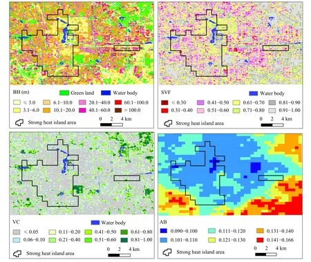
Fig. 9. Distributions of the land-use types, BH, SVF, VC, and AB in the SHI areas and their surrounding areas in Beijing. The black framed areas are the SHI areas.

4.4 Contribution of USL metrics to variations in SUHI and CUHI

Table 4 summarizes the results of the univariate and multivariate stepwise regression analyses between each USL metric and the summer, winter, and annual mean SUHI values. These results are compared with the rates of contribution of each metric to the CUHI (Liu et al.,2021a) in the corresponding time periods.

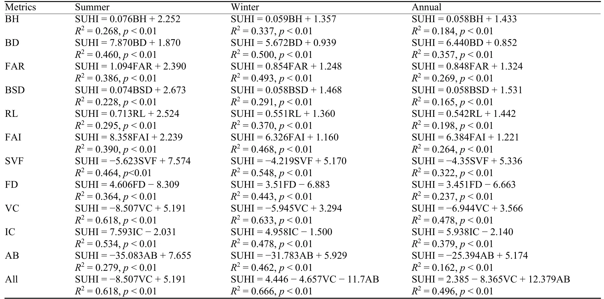
Table 4. Single-factor regression and all-factor stepwise regression models between the summer, winter, and annual mean SUHI values and the USL metrics (BH, BD, FAR, BSD, RL, FAI, SVF, FD, VC, IC, and AB) for Beijing’s CUA in 2009–2018

Analysis of the 11 USL metrics reveals the following.In summer or winter or throughout the year, an increase in BH, BD, and IC or a decrease in SVF, VC, and AB results in an increase in the SUHI (at a significance level of 0.01 for each metric). This pattern is also observed in the impact of each of these factors on the CUHI. In terms of the contribution (R2) of each factor to the variation in the SUHI, each metric individually contributes 16.5%–66.6% of the variation in the SUHI. Except for the IC,each metric individually contributes a larger proportion of the variation in the SUHI in winter than in summer and throughout the year. This finding is nearly the same as that for the CUHI—each metric individually contributes a larger proportion of the variation in the CUHI in winter than in summer and throughout the year. Analysis of the combined contribution of multiple factors to the variation in the SUHI and CUHI reveals the following.The metrics collectively contribute 61.8% of the summer variation in the SUHI, which is higher than the proportion (51.4%) of the summer variation in the CUHI for which they are responsible. In winter and throughout the year, 66.6% and 49.6% of the winter and annual variation in the SUHI, respectively, which are lower than the respective proportions (69.1% and 55.3%, respectively)of the winter and annual variation in the CUHI for which they are responsible.

In summer, VC and IC each contribute more than 50%of the variation in the SUHI, whereas each metric individually contributes less than 50% of the variation in the CUHI. Except for AB, each metric individually contributes more to the variation in the SUHI than to that in the CUHI, suggesting that in summer, most metrics have a greater impact on the SUHI than on the CUHI. Of the 11 metrics, VC, IC, and BD contribute most to the variationin the SUHI. In contrast, BD, VC, and SVF contribute most to the variation in the CUHI in summer. The regression models show that each increase of 10% in VC reduces the SUHI and CUHI by 0.85 and 0.34°C, respectively, and that each decrease of 10% in BD reduces the SUHI and CUHI by 0.79 and 0.37°C, respectively. The multivariate stepwise regression analysis shows that in summer, VC is the primary factor affecting the variation in the SUHI, while BD and AB are the principal factors responsible for the variation in the CUHI.

In winter, VC and SVF each account for more than 50% of the variation in the SUHI. In addition, except for BD, VC, and IC, each metric contributes less to the variation in the SUHI than to that in the CUHI. These findings suggest that in winter, most metrics have a smaller impact on the SUHI than on the CUHI. Of the 11 metrics, VC, SVF, and BD contribute the most (50.0%) to the variation in the SUHI. In contrast, SVF, FAI, and FAR contribute most to the variation in the CUHI. The multivariate stepwise regression analysis shows that VC and AB are the main influencing factors for the variation in the SUHI in winter. In contrast, SVF, AB, and BD are the primary factors affecting the variation in the CUHI.

Annually, VC (47.8%), IC (37.9%), and BD (35.7%)contribute most to the variation in the SUHI, while SVF(45.4%), VC (45.3%), and AB (44.3%) contribute most to the variation in the CUHI. The multivariate stepwise regression analysis shows that annually, VC and AB are the primary factors affecting the variation in the SUHI,while BD, AB, and BSD are the main factors responsible for the variation in the CUHI.

5. Discussion and conclusions

5.1 Discussion

5.1.1Uncertainty in the difference

The SUHI is estimated based on 1-km LST data derived from the imagery taken by the MODIS aboard the Terra and Aqua satellites, while the CUHI is determined by interpolating the temperatures measured at a highdensity network of AMSs to a 1-km grid. The CUA of 1236.7 km2covers approximately 62 urban AMSs with an average distance of nearly 5 km between each station.Moreover, the locations of automatic weather stations are generally in relatively open green spaces (such as parks or green areas) but rarely in building communities, especially high-density and high-rise buildings. Therefore,“forcibly” interpolating the data to a 1-km grid using the spatial interpolation technique does not necessarily reflect the true CUHI at a 1-km resolution. This fact creates a spatial difference between the SUHI and CUHI in addition to some uncertainty in the impact of the USL metrics on them. Therefore, future research should develop a high-resolution numerical simulation technique for the near-surface temperature field that integrates high-resolution building form metrics and perform intensive meteorological observations in some key areas, particularly those with high-density and high-rise buildings, to remedy the current problem associated with the inadequate density of urban meteorological stations.

In addition, the satellite LST data used in this study are all retrieved from imagery acquired by MODIS in the thermal infrared band. LSTs cannot be retrieved from imagery with cloud cover. Therefore, the SUHI values are in fact the mean values for the times with clear weather conditions in each period examined. In contrast, the temperatures recorded at the meteorological stations include those in all clear and nonclear weather conditions. Therefore, the comparison of the SUHI and CUHI has some uncertainty. Hence, it is necessary to further compare the SUHI and CUHI in all weather conditions or only in clear weather conditions to produce more targeted and more scientifically robust results.

5.1.2Uncertainty in the impact

Yang et al. (2011) noted a positive correlation between SVF and CUHI in Shanghai in summer. Yang et al. (2021) also concluded that the SUHI in Hong Kong decreases as SVF decreases during the daytime. These results run counter to the finding of this study that SVF is negatively correlated with the SUHI and CUHI during the daytime in summer (Fig. 7). Generally, SVF has both a positive impact and a negative impact on the CUHI and SUHI. On the one hand, a small SVF results in a large amount of heat in air because solar radiation and refraction of longwave radiation are reflected multiple times by nearby buildings. The accumulated heat, including anthropogenic heat, does not tend to dissipate, resulting in a possible increase in the CUHI or SUHI. On the other hand, due to the blocking effect of buildings, the SVF reduces the received direct solar radiation during daytime and therefore reduces the CUHI or SUHI. The difference between the findings of this study and those of previous studies, as mentioned, may be attributed to two factors.(1) The climate in Beijing differs from that in Shanghai and Hong Kong. The K?ppen climate types in Beijing,Shanghai, and Hong Kong are DWA, CWA, and CFA,respectively. (2) Another important factor is that the meteorological data used in this study are composed of weather data for all clear and unclear weather conditions extracted from a long time series. These data differ considerably from those (data for clear weather conditions only) used in previous studies. Moreover, Wang et al.(2017) noted that IC can explain 31%–38% of the variation in the annual mean SUHI in Beijing, which is close to the finding (37.9%) of the present study, as shown in Table 4, and that IC is strongly correlated with the CUHI at night (IC can explain 49%–54% of the variation in the CUHI) but is not significantly correlated with the SUHI at night. This finding contrasts considerably with the finding of the present study that there exists a strong positive correlation between IC and SUHI at night (Fig. 7).Many studies have found a high level of consistency between the CUHI and SUHI at night (Schwarz et al.,2012; Sun et al., 2015), suggesting that the strong correlation between IC and SUHI at night identified in the present study is more reasonable. This difference is likely related to the methods used to calculate the SUHI and IC and to analyze their spatial correlation performed an analysis based on the area within 1 km of each of 45 stations (Wang et al., 2017), while the analysis in the present study is based on 115 blocks of the whole CUA.Therefore, specific analysis of the difference between the impact of the USL metrics on the SUHI and CUHI requires consideration of weather/climate conditions and of the uncertainty of the data sources and methods.

5.1.3Inconsistency between SUHI and CUHI

SUHIs and CUHIs are formed by different mechanisms. Hence, the SUHI and CUHI are notably inconsistent as indicators of heat islands, particularly daytime heat islands. This inconsistency precludes the application of the SUHI derived from satellite data in a true sense in areas such as urban planning and construction (the CUHI is used as a primary reference metric in practice) and assessment of living environments (e.g., occupant comfort). The difference between the SUHI and CUHI during daytime can be attributed primarily to the following factor. At a fixed angle of observation, a satellite sensor“sees” 2- or 2.5-dimensional mixed urban surface elements (e.g., roofs, one to two building walls, roads, and vegetation), resulting in different heat distribution patterns on the irradiated and shaded surfaces within the sensor’s field of view, which in turn produces a strong“effective anisotropy” in the urban LST. LST can vary by more than 10°C with the direction (Voogt and Oke,1998). This phenomenon is in stark contrast to the uniform temperature “isotropy” due to the sufficient turbulent exchange and mixing of air near the surface during the daytime. To address the problem of LST “anisotropy”due to the inability of satellites to simultaneously observe LSTs in all directions, Voogt and Oke (1997) introduced the concept of a complete surface temperature(CST). CST simultaneously accounts for horizontal and vertical urban surfaces, reflects the thermal effect of three-dimensional urban surfaces, and is a key variable for simulating the surface energy balance, building energy demand, and ensuring occupant comfort. The studies show that SUHI estimates based on measured or simulated CSTs display a daily pattern similar to that of the CUHI (Jiang et al., 2018; Li and Li, 2020). Moreover,compared to LST-based estimates, SUHI estimates based on CSTs simulated from LSTs derived from satellite imagery are more strongly correlated with the CUHI (Yang et al., 2021). However, currently, CSTs are still obtained mainly from surface observations or simulations based on satellite imagery and have yet to be directly determined from satellite imagery in a true sense. Therefore, developing CST-based remote sensing techniques by monitoring SUHIs is an important area of research to address the current inconsistency between SUHIs and CUHIs as indicators of thermal environments.

5.1.4Implications for urban planning

Compared with previous research on UHIs in Beijing,this paper further attains the main USL parameters that affect Beijing’s SUHIs and CUHIs and the differences in their impacts, which are important for heat island mitigation in future urban planning, including the design of some important planning indicators, such as VC, BH,BD, FAI, and AB. In addition, the maximum difference between the CUHI and SUHI is that the CUHI deals with the air in a layer or volume column, not just the air?land interface. Therefore, the formation of CUHIs is more complex than that of SUHIs. It is necessary to consider not only the land surface process but also the horizontal and vertical exchange process of air masses in the air.Moreover, the contribution of all USL parameters to the change in CUHIs or SUHIs is not more than 70%, indicating that there are other important factors affecting the formation of heat islands, such as anthropogenic heat and weather conditions. Therefore, in future urban planning on UHI mitigation, we should consider not only the USL pattern but also the climatic background and local weather conditions, such as wind speed in the wind direction,days of light wind, the frequency or probability of static stability, and temperature inversion weather.

5.2 Conclusions

The SUHI and CUHI differ notably in terms of their distribution patterns and seasonal variation. The difference between their distribution patterns is most pronounced during the daytime in summer. While the SUHI is higher than the CUHI at night, they are highly consistent at spatial and temporal scales at night, particularly in winter, with a spatial correlation coefficient up to 0.80.The SUHI is the highest (5.47°C) at night in winter rather than during the summer daytime, as usually reported.

Spatially, all 11 metrics are strongly correlated with both the SUHI and CUHI at night, with stronger correlations between most metrics and the SUHI. The VC, AB,and SVF metrics have the greatest impact on both the SUHI and CUHI. High SUHI and CUHI values tend to appear in areas with BD ≥ 0.26, VC ≤ 0.09, AB ≤ 0.09,and SVF ≤ 0.67.

In summer, most metrics have a greater impact on the SUHI than on the CUHI, and the opposite is observed in winter. The variation in the SUHI is affected primarily by the VC in summer and by the VC and AB in winter.These main influencing factors differ from those for the CUHI. The metrics collectively explain 61.8% of the spatial variation in SUHI in summer, which is higher than that of CUHI. They contribute to 66.6% and 49.6%of the spatial variation in SUHI in winter and throughout the year, respectively, which are lower than the respective contributions to the variation in the CUHI.