Cho-shui Hn , Xue-zheng Zhu , Jin Gu , Guo-hui Yn , Xio-hui Go ,Qin-wen Zuo

a Institute of NBC Defence, Beijing, China

b State Key Laboratory of NBC Protection for Civilian, Beijing, China

Keywords:Source term inversion Four dimensional variation Observation error regularization factor Bayesian optimization SF6 tracer test

ABSTRACT

1. Introduction

Chemical hazard source term inversion (STI) is the basis of chemical emergency preparedness, emergency response, accident classification and evaluation. In the emergency, the sources of chemical hazard reverse traceability error mainly include the following three aspects: background error, which is caused by complex and changeable environmental factors;observation error,which is caused by different types of observation equipment, instrument error, observation operator error and representative error; model error, whether diffusion model or inversion model has many assumptions and deviates from the actual diffusion law [1].Data assimilation is to quantify, count and minimize the above errors by modifying various parameters in the diffusion model,so as to achieve the purpose of modifying the prediction results of diffusion model and improving the inversion accuracy of source terms, such as Three-Dimensional Variation (3DVAR), Four-Dimensional Variation (4DVAR), Extended Kalman Filter (EKF),Ensemble Kalman Kilter (EnKF), etc. Among them, 4DVAR has attracted extensive attention and application because of its advantages of assimilating multiple continuous time windows and stronger universality [2—6].

For chemical hazard STI, the early research group developed a continuous release multi-sources inversion model based on 4DVAR(FPA-4DVAR STI model)by constructing the adjoint model based on Taylor series upwind difference, background observation error covariance matrix model, equipment observation error covariance matrix model and flower pollination algorithm(FPA) [7,8]. The tracer test shows that although the FPA-4DVAR STI model can effectively improve the inversion accuracy, due to the large deviation between the predicted value of the diffusion model and the real observation value in a small scale, the estimation error of the source term information is still relatively large,so it is necessary to be further improved.

Scholars at home and abroad have carried out a lot of research on the improvement of 4DVAR model. Hendrik Elbern and Hauke Schmidt [9] combined Euler equation with 4DVAR algorithm,increased consideration of chemical reaction and vapor deposition in the diffusion process, and generated an assimilation model suitable for tropospheric trace gas inversion by constructing an adjoint model based on three dimensions: horizontal advection,vertical advection and implicit vertical. After that, they improved the vapor deposition model(RADM2)to generate a new mesoscale air pollution diffusion model and 4DVAR algorithm, which can effectively improve the short-term numerical prediction accuracy of monitored substances [10]. Based on 4DVAR algorithm, Achim Strunk et al.[11]achieved better assimilation performance through grid nesting design, and developed a set of chemical transport model system (EURAD-IM), which can effectively carry out assimilation processing and component analysis of air observation data.Zhang L. et al. [12] constructed a GEOS-Chem adjoint model suitable for fine particle (PM2.5) pollution diffusion based on 4DVAR algorithm, which was verified by the monitoring data of APEC in Beijing in 2014. Liu Yun et al. [13] modified the diffusion model prediction vector in the variational assimilation cost function by using the observation error regularization matrixHa?A,and the STI result is greatly improved compared with that before correction.The disadvantage is that the calculation and statistics of observation error regularization factor was not discussed in detail in the literature,where different statistical methods would have different effects on the correction results. Wang C. et al. [14] integrated the limited memory Broyden Fletcher Goldfarb Shanno algorithm (LBFGS) on the basis of GRAPES-CUACE diffusion model[15—18]and adjoint model [19], and developed a 4DVAR data assimilation system for black carbon emission inversion. The analysis found that the system can reduce the prediction deviation by 1%—36%.

Therefore, based on the former research, aiming at the deficiency that FPA-4DVAR STI model cannot correct the error of diffusion model itself, an improved 4DVAR inversion algorithm with observation error regularization named OER-4DVAR STI model is proposed to further improve the accuracy of chemical hazard STI.Firstly,based on the previous FPA-4DVAR STI model,the OER-4DVAR inversion process and basic inversion model are constructed.Secondly,aiming at the error statistics of chemical hazard diffusion model, the Bayesian optimization method is used toconstruct the observation error regularization factor estimation model.Finally,the scientific,feasible and advanced nature of OER-4DVAR STI model are verified by numerical simulation and tracer test data.

2. OER-4DVAR STI model construction

2.1. OER-4DVAR inversion process

OER-4DVAR STI model is a further improvement of FPA-4DVAR inversion algorithm, whose main idea is divided into the following three stages: after receiving the data reported by reconnaissance equipment or monitoring equipment (longitude and latitude coordinates, altitude, time, hazard type and hazard concentration value), the data terminal separates the prediction error of diffusion model compared with actual hazard concentration at each monitoring point, then the observation error regularization factor(dimensionless)at each monitoring point is obtained by first-order distribution statistics.On this basis,in the face of new emergencies, the predicted concentration correction error can be obtained by multiplying the observation error regularization factor at each monitoring point with the predicted value of diffusion model,and then the predicted concentration correction value with observation error regularization can be obtained. By bringing the corrected predicted concentration value into the 4DVAR inversion model, the concentration prediction vector in the 4DVAR cost function and gradient function is modified, and finally the source term information is estimated. The inversion process of OER-4DVAR is shown in Fig.1.

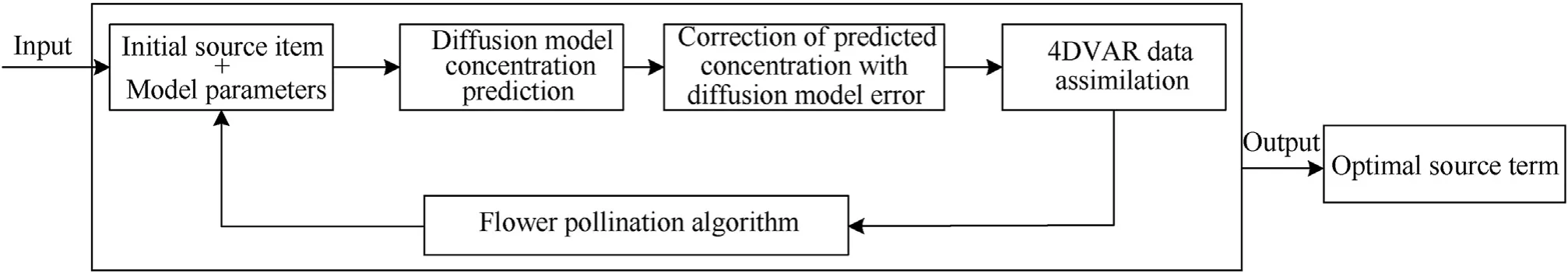
Fig.1. Inversion process of OER-4DVAR.

It can be seen from Fig.1 that the key to the improvement of OER-4DVAR STI model on FPA-4DVAR STI model is to obtain the observation error regularization factor of each monitoring point through the statistical analysis of observation error regularization.Compared with FPA-4DVAR STI model, this method can get the estimation results of source intensity and source location after incorporating the observation error regularization, and the inversion accuracy is higher.

2.2. Basic inversion model of OER-4DVAR

Based on the previous research on multi-point sources FPA-4DVAR STI model, the objective functional and gradient function in the algorithm are modified according to the principle of observation error regularization. Multi point sources FPA-4DVAR STI model is a source intensity and location estimation method proposed by the author in 2021. It considers the release of different locations and multiple hazards, and integrates the Taylor series upwind difference scheme and flower pollination algorithm into 4DVAR model, where its advanced nature has been applied and verified [8]. The model of modified objective functionaland gradient functionis as follows:

where,nis the number of hazard sources; c0is the initial state vector of hazard sources; ci,0is the concentration state vector of hazardous substance at the initial time of theith hazard source;cbis the background field vector; ytis the observation vector of hazardous substance concentration at timet; ′ci,tis the modified state vector of diffusion concentration at timetof theith hazard source;R1is the background observation error covariance matrix;R2is the equipment observation error covariance matrix,which is generally simplified as a diagonal matrix about the error variance of observation equipment; T is the assimilation time window;Dt,Dt-1,…,D1are the tangent linear operators of numerical prediction at each time in the assimilation time window;Htis the observation operator matrix at timet;K-dimensional column vector,Kis the number of monitoring points; R1, R2,HtisK×K-order diagonal matrix.The calculation expression ofis as follows:

where,HaisK×K-order diagonal matrix,whose diagonal element value isHk,t?ci,k,t;Hk,tis the observation operator of monitoring pointkat timet;ci,tis the state vector of diffusion concentration at timetof theith hazard source; Atis the observation error regularization factor vector, At= （a1,t,a2,t,…,ak,t）T;ak,tis the observation error regularization factor of monitoring pointkat timet.

The calculation expression of background observation error covariance matrix R1is as follows:

where,b(x1, x2) is a function of the distancedist（x1-x2） between two points,b（x1,x2） =exp（ -dist（x1-x2）2／2）;?represents Shure inner product;are the predicted concentration state vectors when the prediction time ist= 30 min, and the analysis aging is 10min and 20 min respectively, whose calculation expression are as follows:

where, M30←10and M30←20are the numerical prediction models of 10 min, 20 min—30 min respectively.

3. Observation error regularization factor estimation based on Bayesian optimization

3.1. Separation process of observation error regularization

Observation error regularization refers to the error between the calculated value of diffusion model and the actual observed true value on the premise that the background field, meteorological field and underlying surface are determined.The observation error regularization factor is the dimensionless error factor of the observation error regularization relative to the calculated value of the diffusion model, whose calculation expression is as follows:

where,ak,tis the observation error regularization factor of monitoring pointkat timet;yk,tis the actual observed true value of monitoring pointkat timet;ck,tis the calculated value of diffusion model of monitoring pointkat timet. It can be seen from the observation error regularization factor expression that it reflects the overall error caused by diffusion model itself and all model parameters,which is independently distributed with hazard source term and observation data. Therefore, in order to facilitate the calculation, under the condition of high wind field stability, the dynamic parameter error statistical timeTKis introduced. It is assumed that withinTK, the error factor of diffusion model is only related to the location of monitoring points and has nothing to do with time. InTK, the calculation expression of observation error regularization factor is

where,akis the observation error regularization factor of monitoring pointk;NTKis number of observation times inTK. It can be seen from theakexpression that the selection ofTKhas a great impact on the calculation results, and it should be dynamically adjusted in real time according to the observation interval of nodes and the actual situation on site. If the node observation interval is short and the field data acquisition is relatively simple, the observation error regularization factor at each node can be generated and adjusted in real time according to the collected data. If the node observation interval is long and the actual situation on site is complex, the statistical data of observation error regularization factor at each node can be obtained in advance through pre field test.

3.2. Estimation method for observation error regularization factor

Effective and accurate analysis of observation error regularizations requires a large number of field monitoring data.However,in emergency environment, due to the limitations of strong sudden hazards,small number of monitoring points,short acquisition time and low automation level,there are often few data collected on site,and the data quality also presents“uneven levels”,resulting in large deviation in the calculation results of observation error regularization factors [20]. As a statistical modeling and data analysis method, Bayesian optimization method has the special advantage of quantifying related uncertainty, and can easily fit the complex random effect model that is difficult to be solved by traditional methods, which has been widely used in the fields of solar power generation prediction, diamond surface roughness calculation,monitoring network layout, complex system quantification and so on[21—24].Therefore,based on the Bayesian optimization method,this section screens the data through thedeviation degreeparameter, eliminates the data with largedeviation degree, and then constructs the estimation method of observation error regularization factor. The calculation model ofdeviation degreeis as follows:

where, ξk,tis thedeviation degreeof observation errorregularization factor of monitoring pointkat timet; other parameters are defined as above. Forak,twhosedeviation degreeis greater than the set threshold, a new observation error regularization factorakis obtained by recalculating Eq. (6) after elimination. At the same time, in order to facilitate statistical calculation,the data of observation error regularization factor are divided into“good data”, “general data” and “bad data” according to the deviation degree[25,26]. The evaluation criteria are shown in Table 1.

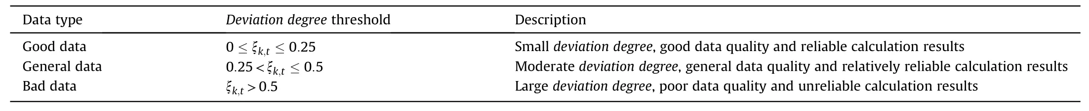
Table 1Evaluation criteria of observation error regularization factor data.

It can be seen from Table 1 that“good data”is closer to the actual observation and the calculation results are more reliable.However,in the field environment, “good data” is often a small amount and more “general data”. How to make good use of “good data” and“general data” is very important to obtain reliable calculation results.Therefore,based on Bayesian estimation,“good data”is taken as the prior distribution information of observation error regularization factor, and the likelihood function is calculated through“general data”.Assuming that the observation error regularization factor obeys the normal distribution, then the calculation expression of mean μaand standard deviation σafor posterior distribution is as follows:

where,μpis the mean of the priori distribution; μlis the mean of likelihood function; σpis the standard variance of the priori distribution;σlis the standard variance of likelihood function.In order to further improve the stability and accuracy of the calculation results, referring to the research of Anders Kristoffersen [27] and Trichtinger L.A. [28], it is set that the observation error regularization factor obeys the lognormal distribution, and then the calculation expression of mean μauand standard deviation σaufor posterior distribution is as follows:

The parameter definition is the same as above. Therefore,through Eq.(5)to Eq.(9),the estimated value of observation error regularization factor of each monitoring point can be obtained.

3.3. Parameter definition of OER-4DVAR STI model

In order to facilitate model calculation and algorithm compilation, the objective function, source term parameters, intermediate variables and basic parameters involved in OER-4DVAR STI model are defined, as shown in Table 2.

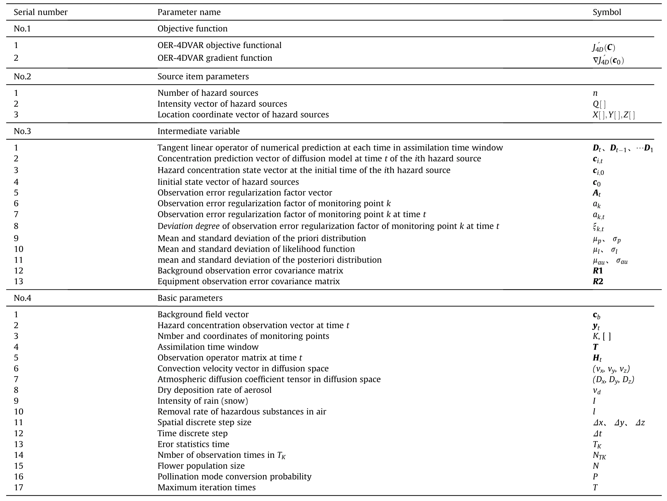
Table 2Parameters of OER-4DVAR STI model.

4. Numerical simulation analysis

In order to verify the scientific nature and feasibility of OER-4DVAR STI model, the algorithm is verified by numerical simulation in two cases of two point sources and four point sources.

4.1. Initial condition setting

The initial conditions mainly include the inversion model parameters and the layout scheme of monitoring points. Set the parameters according to the definition of model parameters in Section 2.3, as shown in Table 3.

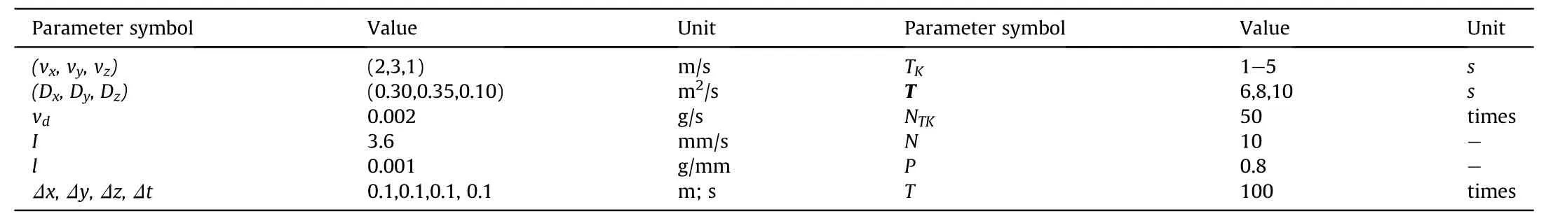
Table 3Parameter setting table of OER-4DVAR STI model.

According to the layout requirements of dense in front and sparse in back and uniform arrangement [29,30], 30 points with a height of 2 m and regular distribution are selected as monitoring points, where the layout scheme of monitoring points is shown in Fig. 2. In order to more intuitively analyze the feasibility of this algorithm,it is assumed that the background error and observation error of each monitoring point are in a standard normal distribution in the numerical simulation, and the background observation error covariance matrix R1and equipment observation error covariance matrix R2are simplified as diagonal matrix.

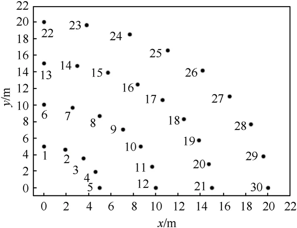
Fig. 2. Layout plan of monitoring points.

Next, the analytical solution data at each time plus 10%—50%random interference is used as the observation data of hazard concentration, and the source intensity and location of two point sources and four point sources are estimated respectively through OER-4DVAR STI model. The calculation expressions of source intensity estimation error δintension, source intensity estimation relative error εintension, location estimation error δlocation and location estimation relative error εlocation are as follows:

where,nis the number of hazard sources;Qi1is the estimated value of intensity for theith hazard source;Qi0is the real value of intensity for theith hazard source; （xi1,yi1,zi1） is the location estimation coordinate of theith hazard source; （xi0,yi0,zi0） is the real location coordinates of theith hazard source.

4.2. Case of two point sources

The source item information is set as follows: the number of hazard sources is 2, the source intensity vector Q = [5,8], and the location coordinate vector {X, Y, Z} = { [1,3,3,3,3,5]}. According tothe steps in Section 2.1, 50 groups of error statistical data are classified and distributed, and the estimated values of observation error regularization factors of 30 monitoring points are obtained,as shown in Table 4.

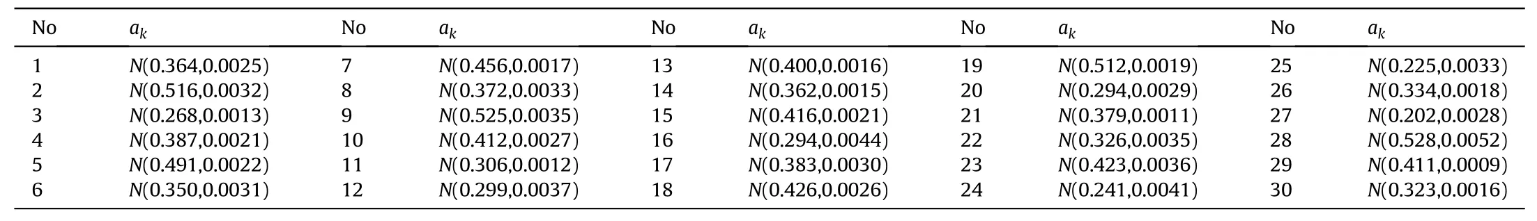
Table 4Observation error regularization factor estimation results of monitoring points.

Based on the estimation of observation error regularization factor, the source term information is estimated and the error is calculated through the OER-4DVAR STI model. The inversion assimilation curve is shown in Fig. 3.

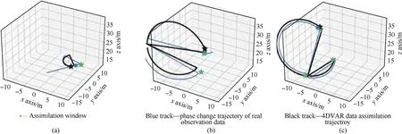
Fig. 3. Inversion assimilation curve of two point sources: (a) t = 6 min; (b) t = 8 min; (c) t = 10 min.

In Fig. 3, the green Pentagram represents an assimilation node,the blue curve represents the phase transition trajectory of observed data, the black curve represents the phase transition trajectory of predicted data after OER-4DVAR assimilation,the blue solid dot represents the final phase transition position of observed data in the assimilation window, and the black Pentagram represents the final phase transition position of predicted data in the assimilation window. It can be seen from Fig. 3 that in the case of two point sources, the phase change trajectory of predicted data after three assimilations is basically consistent with that of observed data. From the second assimilation window, the final position of phase transition between the predicted data and the observed data basically coincides, indicating that OER-4DVAR shows good results in assimilation and inversion. In order to better analyze the inversion effect, the inversion results of OER-4DVAR, 4DVAR and FPA-4DVAR are compared and analyzed, as shown in Table 5.Parameters setting of 4DVAR and FPA-4DVAR are the same as that of OER-4DVAR.

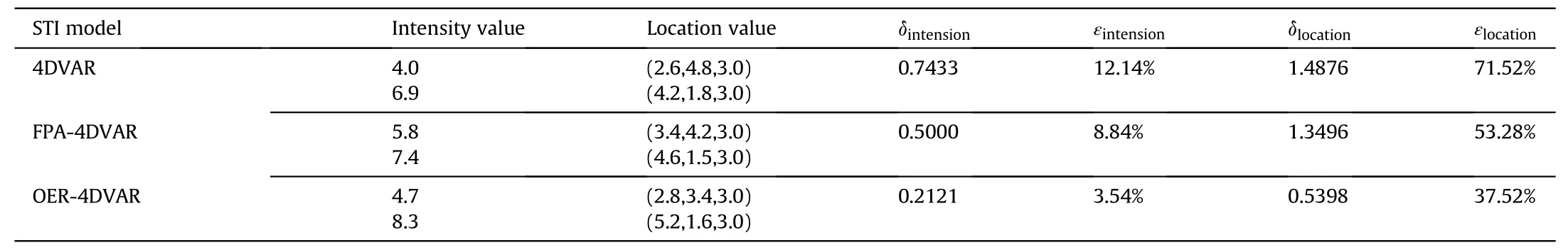
Table 5STI results of two point sources.

4.3. Case of four point sources

The source item information is set as follows: the number of hazard sources is 4, the source intensity vector Q = [3,5,8,10], and the location coordinate vector {X, Y, Z} = { [1,3,5,7], [1,3,5,7][3,3,3,3]}. According to the steps in Section 2.1, 50 groups of error statistical data are classified and distributed, and the estimated values of observation error regularization factors of 30 monitoring points are obtained, as shown in Table 6.

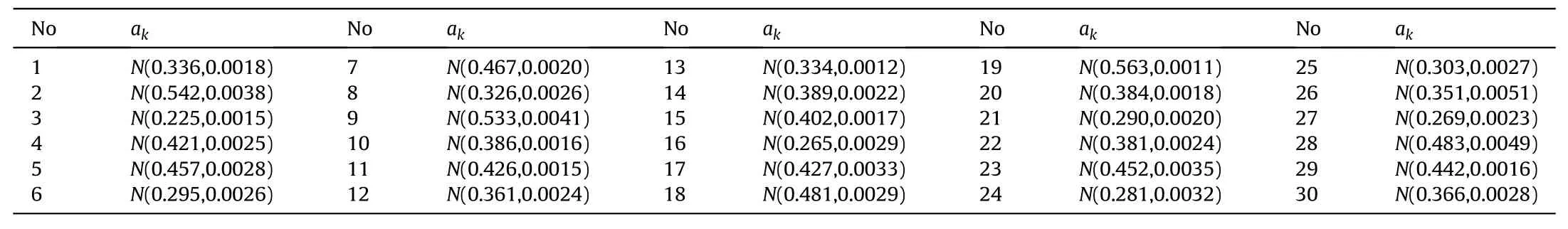
Table 6Observation error regularization factor estimation results of monitoring points.

Based on the estimation of observation error regularization factor, the source term information is estimated and the error is calculated through the OER-4DVAR STI model. The inversion assimilation curve is shown in Fig. 4.

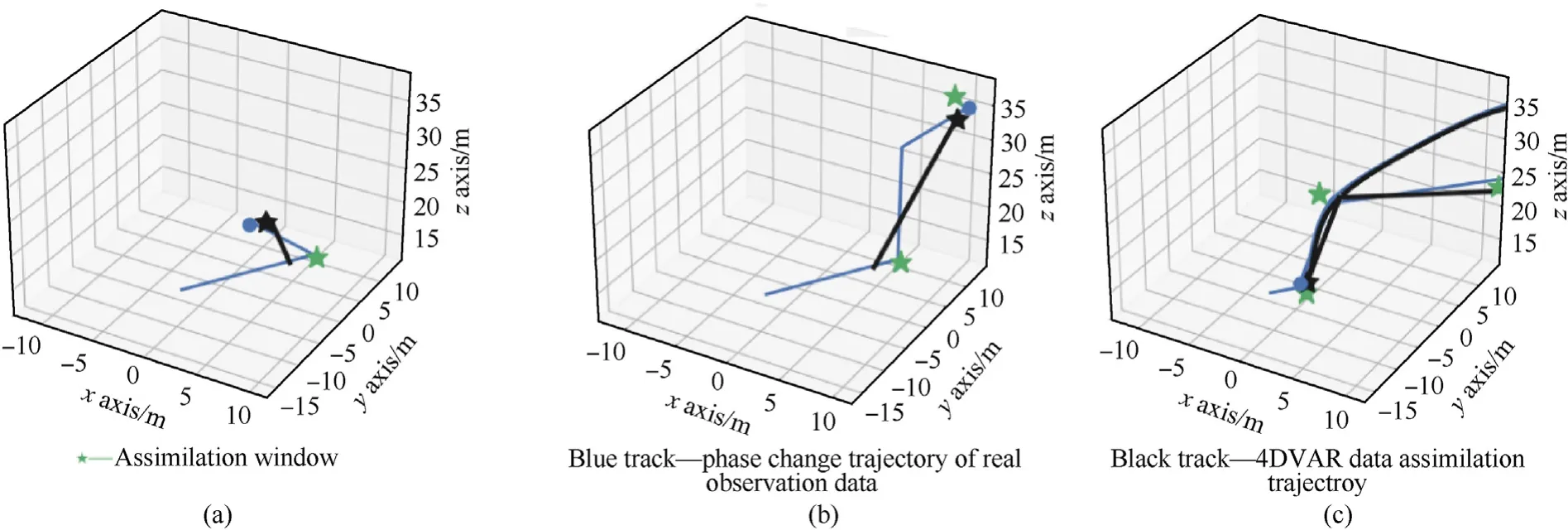
Fig. 4. Inversion assimilation curves of four point sources: (a) t = 6 min; (b) t = 8 min; (c) t = 10 min.

It can be seen from Fig. 4 that in the case of four point sources,the phase change trajectory of predicted data after the first two assimilations is quite different from that of observed data, and it does not become basically consistent until the third assimilation window,and the assimilation effect is reduced compared with the case of two point sources. After three times of OER-4DVARassimilation, the final position of phase transition between predicted data and observed data basically coincides, indicating that OER-4DVAR still has good inversion performance in this case. The inversion results of OER-4DVAR, 4DVAR and FPA-4DVAR are compared and analyzed, as shown in Table 7.

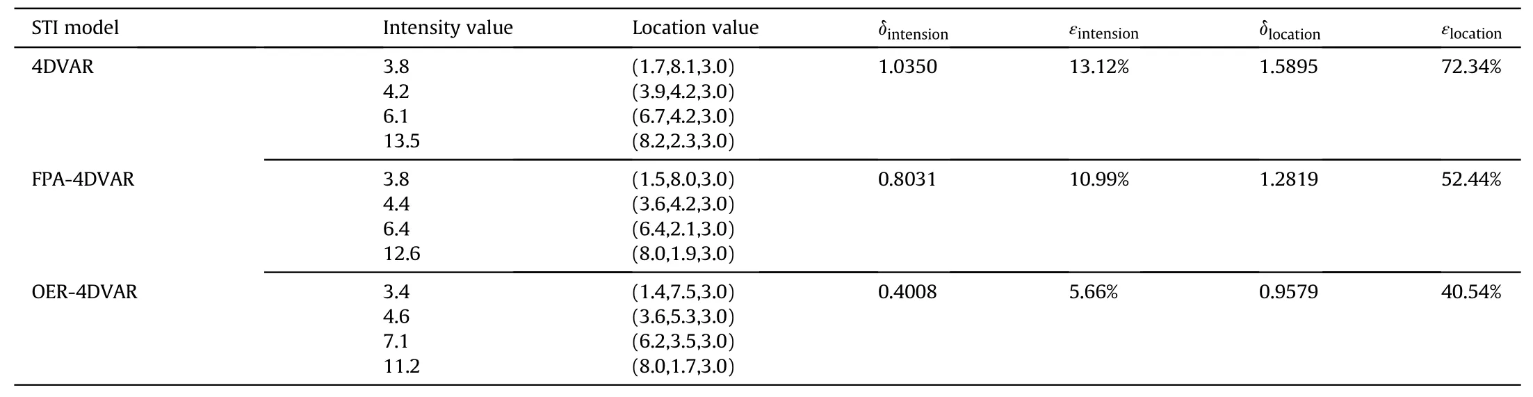
Table 7STI results of four point sources.

It can be seen from Table 7 that for the case of four point sources,the source intensity and location estimation results of OER-4DVAR are still closer to the real value. Compared with FPA-4DVAR, after using observation error regularization, the relative error of source intensity estimation is reduced from 10.99% to 5.66%, and the relative error of location estimation is reduced from 52.44% to 40.54%. The inversion effect is improved to a certain extent.

Based on the SIT in the two source term cases,whether it is two point sources or four point sources, the inversion results of OER-4DVAR are improved to a certain extent compared with 4DVAR and FPA-4DVAR. At the same time, with the increase of the complexity of the source term case, the inversion error of OER-4DVAR increases, but it does not diverge. In addition, the estimated values of observation error regularization factor at the same monitoring point and different hazard sources are different,but basically close,which is caused by the response degree floating of each monitoring point under different source terms,resulting in fluctuations in the estimated value of observation error regularization factor.The random errors of different statistical samples are also an important reason for this situation. Therefore, in practical application,the statistical results of different cases can be fused to further improve the credibility of the estimation results.

5. Verification of tracer test data

To further analyze the feasibility and advanced nature of OER-4DVAR STI model, the 10 SF6tracer diffusion tests conducted in Cangzhou, Hebei in from May 21 to 24, 2016 are taken as an example to verify.The ownership of test data belongs to the project team.The 1st,3rd,5th,7th and 9th test data with high atmospheric stability are selected as the estimation samples of observation error regularization factor, and the 2nd, 4th, 6th and 8th test data are selected as the test samples to verify and compare the 4DVAR,FPA-4DVAR and OER-4DVAR STI models respectively.

5.1. Basic information of tracer test

The space of tracer test site is about 10 × 7 km2, and the coordinates of release points are(8406 m,6322 m)in meters.A total of 4 fixed meteorological stations, 20 portable meteorological monitoring points and 50 fan-shaped concentration sampling points are set up to observe the data of wind speed, temperature,humidity, air pressure and tracer concentration in real time.Considering the accessibility of distribution points, availability of data and other factors,semi-circular distribution shall be arranged at 0.5 km,1 km and 2 km of the release point as far as possible,and different sampling arcs shall be arranged at the downwind distance of about 3 km, 5 km, 7 km and 10 km. As the area near the study area is a nature reserve,mostly reed swamp terrain, and there is a salt field in the distance (no sampling personnel are allowed), It is difficult to form a coverage monitoring area. The layout of monitoring nodes is shown in Fig. 5.

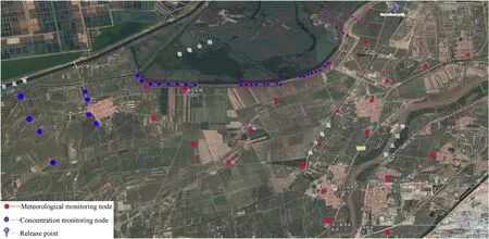
Fig. 5. Layout scheme of monitoring nodes.

In the actual release process, the release height of the 1st-3rd,6th, 7th and 10th tests is 100 m,and the release height of the 4th,5th, 8th and 9th tests is 30 m. The SF6release and simulation conditions are shown in Table 8.SF6samples were collected by EM-1500 portable gas sampler and LB-201-4 L aluminum foil sampling bag, and analyzed by Shimadzu GC-2010 gas chromatograph. The sampling time interval is 10 min.

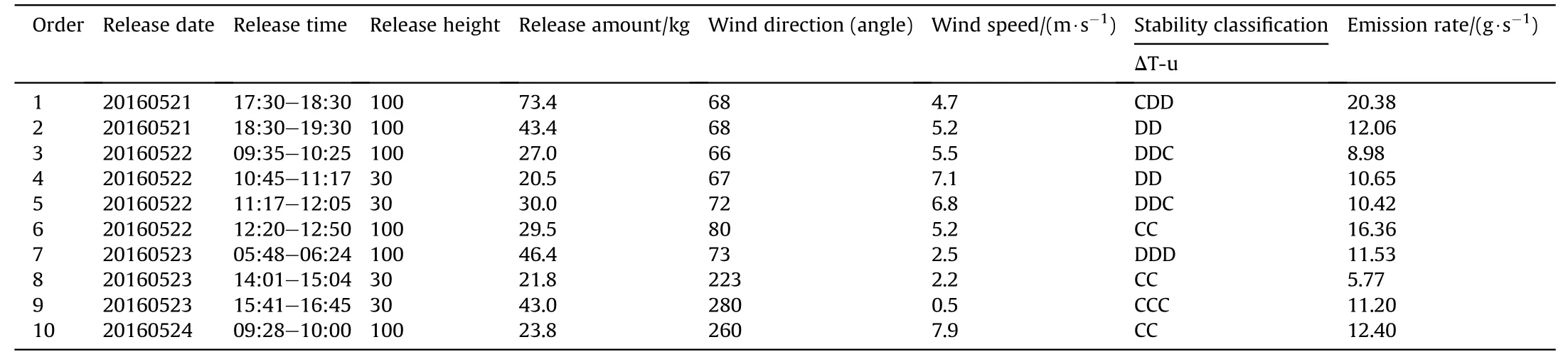
Table 8SF6 tracer experiment and simulation conditions.

Next, take the 1st, 3rd, 5th, 7th and 9th times test data as training samples to estimate the observation error regularization factor of each monitoring point,and take the 2nd,4th,6th,8th and 10th test data as test samples to verify the OER-4DVAR STI model.

5.2. Estimation of observation error regularization factor

According to the observation error regularization factor estimation method in Section 2, the observation error regularization factor of each monitoring point at each time in the five tests are calculated respectively. The mean and variance of the observation error regularization factor of each monitoring point are obtained through data separation, priori distribution, likelihood function distribution and posteriori distribution, as shown in Table 9.

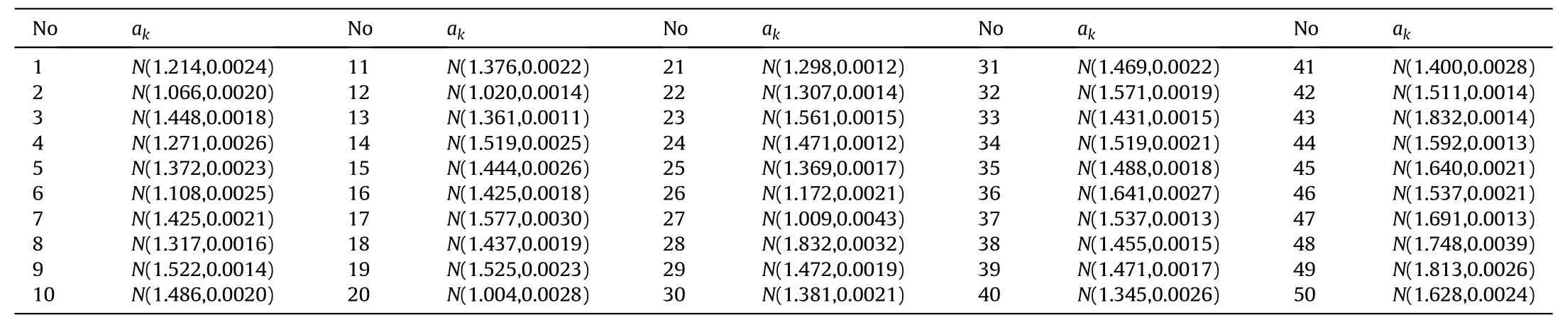
Table 9Observation error regularization factor estimation results of monitoring points.

It can be seen from Table 9 that in the field tracing test,the mean value of the error factor between the diffusion prediction results and the actual observation results of each monitoring point is maintained at 100%—200% (Fig. 6(a)). The variance of observation error regularization factor at each monitoring point is maintained between 0.0011 and 0.0043 (Fig. 6(b)). From the perspective of spatial distribution, the mean value of observation error regularization factor increases gradually with the increase of number (the farther away from the release source),indicating that the influence of meteorological information and background information on concentration prediction increases gradually with the increase of distance. From the perspective of time-varying characteristics,except for node 27 and node 48, the error factor variance of diffusion model does not diverge with the increase of distance,and the variation interval is relatively stable, indicating that the statistical results of five training samples have little difference,which can be used for the test of OER-4DVAR STI model.

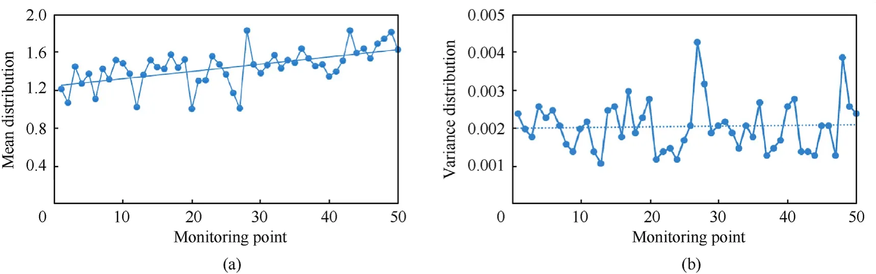
Fig. 6. Distribution map of observation error regularization factor estimation at each monitoring point: (a) Observation error regularization factor mean distribution; (b) Observation error regularization factor variance distribution.

5.3. Estimation of source intensity and location

The OER-4DVAR STI model is set as follows: ①the source location and intensity are unknown;②the spatial step size,the number of spatial steps,the time step size and the number of time steps m are determined by the specific test conditions; ③air is set as the main phase and SF6as the second phase, σx, σy, σzare calculated according toP-Gdiffusion curve; the density of SF6is 6.52 kg/m3and the dynamic viscosity is 0.0000142 pa?s; ④flower population sizeN= 200, pollination mode conversion probabilityP= 0.8,maximum iteration timesT= 500. Taking the second test as an example, the release source strength and source position are inversely estimated through the monitoring data at each time and OER-4DVAR STI model. The parameter settings of the inversion algorithm are shown in Table 10.

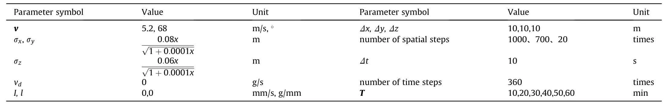
Table 10Parameter setting table of 2nd test.

The inversion assimilation curve is shown in Fig. 7.

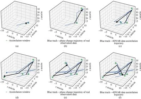
Fig. 7. STI assimilation curve of the second tracer test: (a) t = 10 min; (b) t = 20 min; (c) t = 30 min; (d) t = 40 min; (e) t = 50 min; (f) t = 60 min.

It can be seen from Fig. 7 that after assimilation of six time windows, the predicted data and observed data are basically consistent from the initial chaotic state, showing a good inversion effect, regardless of the phase transition trajectory or the final position of the phase transition.The STI results based on OER-4DVAR are shown in Table 11.

Table 11STI results based on OER-4DVAR.

5.4. Analysis of experimental results

5.4.1. Advantages and disadvantages analysis of OER-4DVAR

Referring to the 2nd times test analysis,analyze the test data of the 4th, 6th, 8th and 10th times in turn to obtain the source intensity and location information under each test sample.In order to better analyze the improvement effect of OER-4DVAR STI model,compare it with 4DVAR and FPA-4DVAR,verify its advanced nature and accuracy improvement degree, as shown in Table 12.

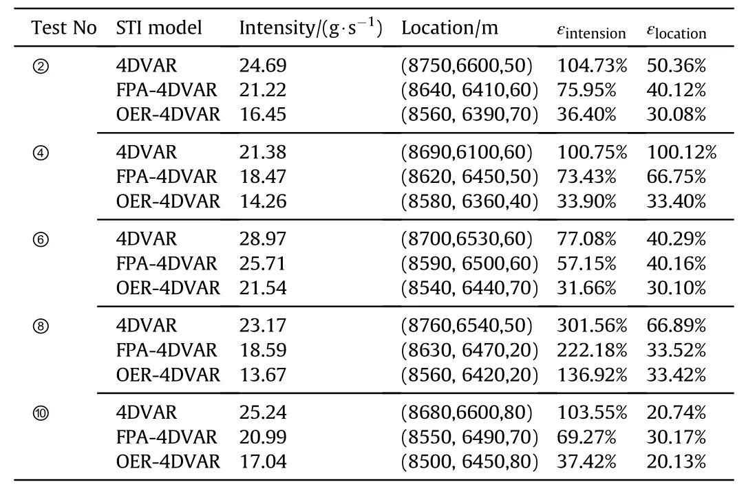
Table 12Comparison among 4DVAR, improved 4DVAR and OER-4DVAR.

Fig.8 is a comparison diagram of the calculation results and true values of source intensity, source height, horizontal location and location relative error respectively.

It can be seen from Table 12 and Fig. 8 that the traceability accuracy of 4DVAR inversion algorithm is significantly improved by introducing the observation error regularization factor. Compared with the ordinary 4DVAR inversion algorithm,the source intensity estimation accuracy of OER-4DVAR STI model is improved by about 61.80%,and the source location estimation accuracy is improved by about 37.03%. Compared with FPA-4DVAR STI model, the source intensity estimation accuracy of OER-4DVAR STI model is improved by about 46.97%, and the source location estimation accuracy is improved by about 26.72%. At the same time, the estimation errorof source intensity in the eighth test is significantly higher than that in other tests. This is due to the small release of tracer in this test and the significant convection effect in the air, which leads to the failure of collecting effective data at many monitoring points.

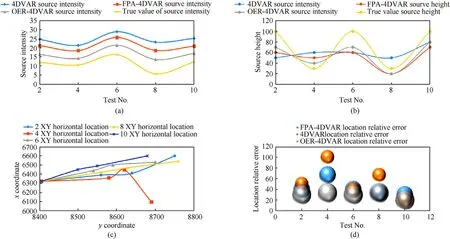
Fig. 8. Comparison of STI results: (a) Results of source intensity; (b) Results of source height; (c) Results of horizontal location; (d) Results of location relative error.

5.4.2. Error cause analysis

According to the verification of tracer test data,the OER-4DVAR STI model can effectively solve the intensity and location of hazard sources,and the accuracy is significantly improved compared with ordinary 4DVAR and FPA-4DVAR. However, there are still some cases where the inversion error is large. The main reasons can be divided into the following aspects:

(1) Background error analysis

During the tracer test,the atmospheric stability is mostly C and D, the wind speed is mostly about 5—7 m/s, the diffusion space is located in the weak low pressure field, the isobaric line is sparse,the pressure gradient is weak,the terrain of the diffusion site is flat,and the influence of topographic circulation is very small. Therefore, the influence of background error on the inversion results is relatively small.

(2) Observation error analysis

Observation errors are mainly caused by instrument errors of different types of observation equipment, observation operator errors and representative errors. The equipment and instruments used in this test have been calibrated by the calibrator, but due to the limitation of sampling height and sampling area, they are not arranged according to the requirements of dense in front and sparse in rear and uniform arrangement.There are obvious building interference near some points, which has become an important factor leading to calculation error.

(3) Model error analysis

Although the introduction of observation error regularization factor can effectively reduce the impact of observation error regularization, due to the polymorphism of atmospheric environment and too many external disturbance factors, both diffusion model and inversion model still have large deviation from the actual diffusion law, and the improvement of STI accuracy is limited.It is necessary to further modify and adjust the calculation model through a large number of test data.

5.4.3. Algorithm applicability analysis

Through the tracer test analysis, the algorithm established in this paper can better reverse calculate the hazard source term information under the conditions of high atmospheric stability and flat underlying surface. In practical work, on this basis, combined with ground mobile reconnaissance equipment and unmanned reconnaissance equipment, we can further develop ground reconnaissance and search, and build an accurate traceability mode combining active and passive.

6. Conclusions

By introducing the observation error regularization factor based on Bayesian optimization, this paper further improves the FPA-4DVAR STI model, and generates a new STI algorithm named OER-4DVAR.According to the numerical simulation and tracer test data verification, the following conclusions are obtained: (1)compared with ordinary 4DVAR and FPA-4DVAR STI models, OER-4DVAR STI model has obvious advantages in the inversion of source intensity,source height and abscissa and ordinate;(2)OER-4DVAR STI model requires high training sample size, which needs to be corrected and adjusted through a large number of experiments in practical application; (3) this paper mainly applies OER-4DVAR STI model to Gaussian diffusion model. Next, the fusion and optimization between it andk-ε turbulent model or randomwalk particle-puff model will be studied.

Funding

Thank the Ministry of Science and Technology of the People's Republic of China for its support and guidance (Grant No.2018YFC0214100).

Data availability statement

The data used to support the findings of this study are available from the corresponding author upon request.

Code availability

(software application or custom code): Not applicable.

Declaration of competing interest

The authors declare that they have no known competing financial interests or personal relationships that could have appeared to influence the work reported in this paper.