Zhi-Xin Li·Qing-Jie Cao·Alain Léger

?

The equilibrium stability for a smooth and discontinuous oscillator with dry friction

Zhi-Xin Li1·Qing-Jie Cao1·Alain Léger2

?The Chinese Society of Theoretical and Applied Mechanics;Institute of Mechanics,Chinese Academy of Sciences and Springer-Verlag Berlin Heidelberg 2015

AbstractIn this paper,we investigate the equilibrium stabilityofaFilippov-typesystemhavingmultiplestickregions based upon a smooth and discontinuous（SD）oscillator with dry friction.The sets of equilibrium states of the system are analyzed together with Coulomb friction conditions in both （fn,fs）and（x,˙x）planes.Inthestabilityanalysis,Lyapunov functionsareconstructedtoderivetheinstabilityfortheequilibrium set of the hyperbolic type and LaSalle’s invariance principle is employed to obtain the stability of the nonhyperbolic type.Analysis demonstrates the existence of a thick stable manifold and the interior stability of the hyperbolic equilibrium set due tothe attractive slidingmode ofthe Filippovproperty,andalsoshowsthattheunstablemanifolds ofthehyperbolic-typearethatoftheendpointswiththeirsaddle property.Numerical calculations show a good agreement with the theoretical analysis and an excellent efficien y of the approach for equilibrium states in this particular Filippov system.Furthermore,the equilibrium bifurcations are presented to demonstrate the transition between the smooth and the discontinuous regimes.

KeywordsSD oscillator·Equilibrium set·Dry friction· Coulomb’s cone

1　Introduction

Dry friction induced dynamics has attracted the attention of researchersformanyyears［1-5］,whichismotivatedbyengineering applications［6］.The presence of dry friction can affect the behavior and the performance of mechanical systems as it can induce complex phenomena,such as periodic motion［7］,stick-slip vibrations［8,9］,etc.Many mechanical systems experience stiction due to dry friction which may induce the existence of equilibrium sets of intervals,rather than the isolated equilibria.Moreover,the stability property of the equilibrium set can dramatically affect the entire dynamics performance of the mechanical systems［10］.In Ref.［11］,the sufficien conditions for attractivity and unstability of the equilibrium sets were given by employing the Lyapunov stability theory and Lasalle’s invariance principle. The stability properties of the equilibrium set for the nonsmooth dynamic systems can be determined by Lyapunov stability theory［12,13］.By using the Coulomb friction law, the set of equilibrium states of a mass-spring system with unilateral contact and Coulomb friction were investigated, and the stability properties of all these equilibrium states are obtained with numerical experiments in Ref.［14］.In addition,thebifurcationoftheequilibriumsetforthenon-smooth systems with dry friction are studied in Ref.［15］.Filippov ［16］firstl provedthatthesystemswithdryfrictiondescribed bydifferentialequationswithadiscontinuousright-handside can be extended to differential inclusions［17］with a set valued right-hand side,which is often called the Filippov-type systems.Leine［18］foundthatthestablemanifoldofaunstable equilibrium set is“thick”in a constrained bar system of Filippov-type,but did not make an explanation for this mechanism.

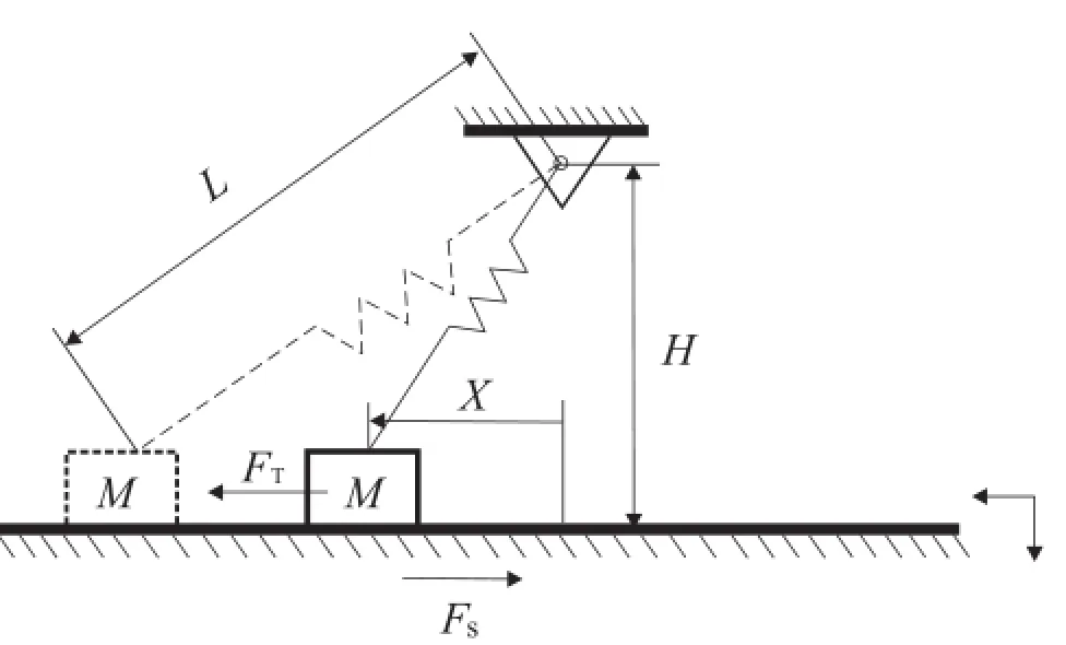
Fig.1 SD oscillator with dry friction

A smooth and discontinuous（SD）oscillator［19-21］is an archetypegeometricalnonlinearsystem,whichdemonstrates theunificatio andthetransitionbetweenthesmoothanddiscontinuous dynamics.The restoring force of this oscillator has an irrational term,which is often called the irrational nonlinearity demonstrating both geometrical and physical properties of the system［22］.The system may have three equilibria（0≤α＜1）or a single equilibrium（α≥1）［19］.The corresponding equilibria might be extended into equilibrium intervals when the system is subjected to the dry friction,which has been investigated in Ref.［23］using Coulomb’s cone.

The motivation of this paper is to investigate the stability of the equilibrium sets for the SD oscillator with dry friction byusingFilippov’stheorytogetherwithLyapunov functions andtheLasalle’sinvarianceprinciple.Anothermotivationof this work is to illustrate the mechanism of the unstable equilibrium set having the thick stable manifold［18］due to the attractiveslidingmodeoftheFilippovproperty.Wefocusour attention on the constructing of the sets of equilibrium states for this system with the help of Coulomb’s cone,the proof of the instability for the equilibrium set of hyperbolic type, the stability of the equilibrium set of non-hyperbolic type, the property of the sliding mode［24］,and the equilibrium bifurcation phenomena of this system.

2　The mechanical model

Consider the mechanical model as shown in Fig.1,in which a mass M is attached to a fi ed point via a inclined linear spring of stiffness K being capable of resisting both tension and compression.It is supposed that the mass is restricted in the surface moving horizontally.We denote the horizontal positionofthemassby X anditsvelocityby˙X.Thefrictionis modeled by Coulomb’s law,which is opposite to the relative velocity between the mass and surface.

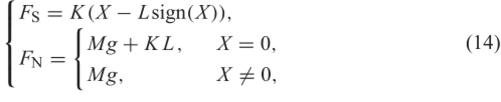
The equation of motion reads from Newtow’s second law where is the horizontalforceexe rted on th e massb yt hes pring. L and H representthe original length of the spring and the distance between fi ed point and surface,respectively.FSdenotes the friction force between the mass and surface,which satisfie the following Coulomb friction condition,

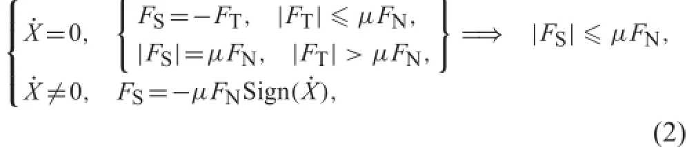
where

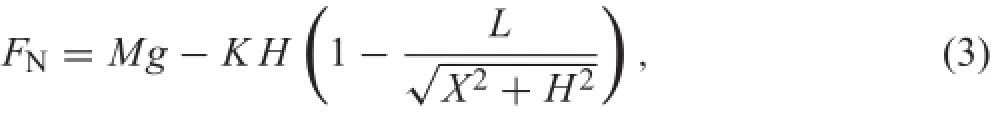
which is the total contact force of the gravity of the mass and vertical component of the spring force to be assumed so that the direction of FNalways points down（FN＞0）.sign（·）is the signum function,g is the gravitational acceleration and μ is the friction coefficient

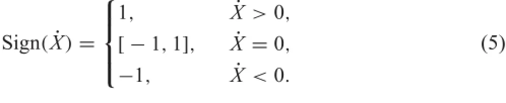
From Eq.（2）following the set-valued force law［11］,we obtain

where the set valued function Sign is given by

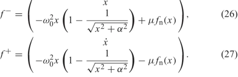
The corresponding non-dimensional equation of motion together with Eqs.（1）and（4）is formulated by employing the differential inclusion of Filippov-type［16］:

where

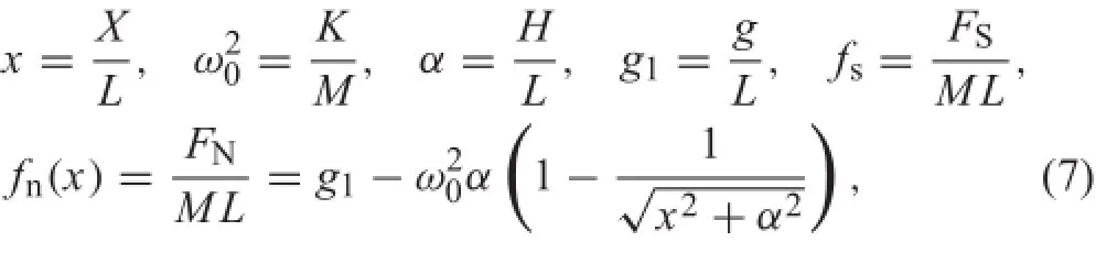
furthermore,

It is noted that friction fs（x,˙x）is not only relevant to the velocity˙x,but also the position x concerned,since themagnitude of friction varies with displacement,as shown in Fig.2,in which the thick solid curve presents the friction force fs（x,˙x）when˙x=0.

Fig.2 Schematicdiagramoffriction fs（x,˙x）forthesystem（6）,which depends on the velocity˙x and position x.The thick solid curve presents the friction force fs（x,˙x）when˙x=0

3　The set of equilibrium states

TheCoulombfrictionconditions（2）showninFig.3aimplies that the mass can slip only when the friction force FShas attained one end of the interval（?μFN,μFN）,and when it slips its velocity and the friction force FSare of opposite sign,and the mass can stick when the friction force FSmust belong to the interval（?μFN,μFN）.By combining these conditions we can see that the friction force FSmust belong to the the cone（gray area of the Fig.3b）in（FS,FN）plane, referred to as the Coulomb’s cone［25］.

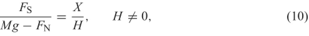
We are interested in looking for the equilibrium states of the system,which can be obtained together with the conditions FS=?FTfor˙X=0 in Eqs.（2）and（3）

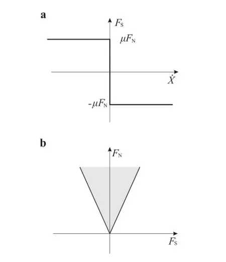
Fig.3　a Coulomb friction conditions in（˙X,FS）plane.b Coulomb’s cone in（FS,FN）plane

Substituting Eq.（11）into Eq.（10）it follows that

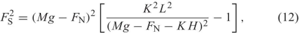
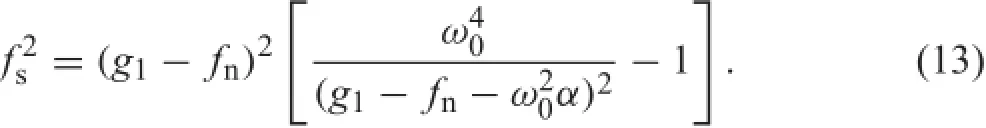
which can be rewritten in the following form according to the expressions in Eq.（7）.

In particular,we shall comment on the equilibrium solutions on the situation α=H/L=0.Thus,the equilibrium equationcanbealsogivenbycombiningthesameconditions FS=?FTfor˙X=0 in Eqs.（2）and（3）

which takes form by using the expression（7）as following

which leads to

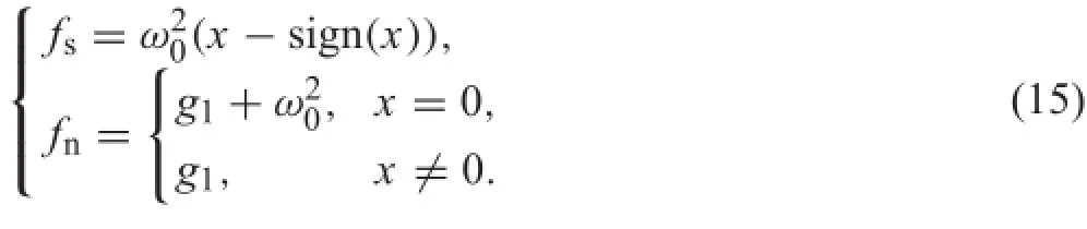
then follows

Figure 4 shows the corresponding equilibrium solutions in（fs,fn）plane with respect to the value of the parameter α.The thick black lines are the boundaries of the Coulomb’s cone（?μfn≤fs≤μfn）,and the solutions of equilibriumare given by the intersection of the red curves（13）（α＞0）and（15）（α=0）with the part of the Coulomb’s cone.In Fig.4a,there are three sets of equilibrium states for this system when 0＜α＜1,and only one set of equilibrium states exists when α=1,as shown in Fig.4b.If α=0, there are two sets of equilibrium states in the stick state（two straightlinesoverlapduetothesymmetryofthissystem）and one solution in the impending slip state,and this situation is denoted on Fig.4c.

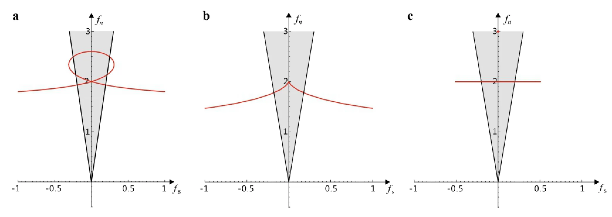
Fig.4　The sets of equilibrium states in（fs,fn）plane.a 0＜α＜1.b α=1.c α=0

Eventhesetsofequilibriumstatesforthissystemaregiven in（fs,fn）plane,wewilltransformtheequilibriumstatesinto （x,˙x）planefortheconvenienceinthefollowingsections.An equilibriumset,beingaconnectedsetofequilibriastickingin all contact points,can be described by using the differential inclusion.

The equilibrium set of the system（6）is given by

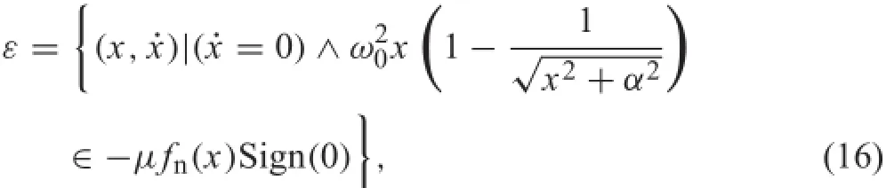
where the Sign（0）is taken as the whole interval［?1,1］,as define in Eq.（5）.

The SD oscillator with dry friction shows that there exists three isolated equilibrium sets for 0＜α＜1:

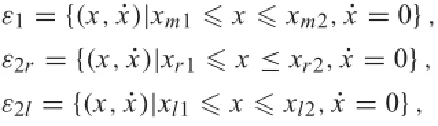
which are marked with thick solid lines in Fig.7,where xm1, xr1,and xl1are left endpoints of the equilibrium sets ε1,ε2r, andε2lrespectively,xm2,xr2andxl2arerightendpointsofthe equilibrium sets ε1,ε2r,and ε2l,respectively,furthermore, xm1=?xm2,xr1=?xl2,and xr2=?xl1.

Furthermore,when α=0,there exists one equilibrium point（0,0）andtwoisolatedequilibriumsetsforthissystem:

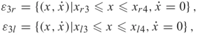
which are indicated by thick solid lines in Fig.8a,where xr3and xl3are left endpoints of the equilibrium sets ε3rand ε3l, respectively,xr4andxl4arerightendpointsoftheequilibrium sets ε3rand ε3l,respectively,furthermore,xr3=?xl4and xr4=?xl3.

When α=1,this system shows that there exists only one equilibrium set

marked by a thick solid line,as shown in Fig.8b,where xl5and xr5are the left endpoint and right endpoint of the equilibrium set ε4,respectively,and xl5=?xr5.

It is easily verifie that the sets of equilibrium states in （fs,fn）plane correspond to the equilibrium sets in（x,˙x）planeforthissystemwithrespecttothevalueoftheparameter α,since the equilibrium solutions in（fs,fn）plane and in （x）plane can be transformed into each other by using the Eqs.（13）（α＞0）,（15）（α=0）and the set（16）.At the same time,it has been shown that the system（6）exhibits not only the bifurcation of equilibrium states in（fs,fn）plane, but also the bifurcation of equilibrium sets in（x,˙x）plane,in terms of the value of the parameter α.

4　Stable analysis of equilibrium set

In this section,we will discuss the stability of all the equilibriumsetsoftheSDoscillatorwithdryfriction.Inthissystem, x=（x,˙x）T∈R2.

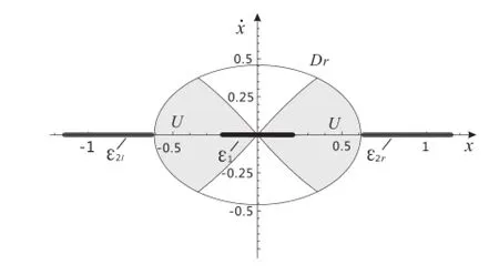
Fig.5　Schematic representation of the set U（shown in grey）in which V≥0（V as in Eq.（18））

4.1Instability analysis of the equilibrium set ε1

Wenowstudythestabilitypropertyoftheequilibriumsetε1. Firstly,let us introduce the following theorem:

Theorem 1（instability theorem for equilibrium sets［18］）Let ε be a bounded connected equilibrium set of the differential inclusion, withRn,F:RnRn.Let V（x）be a continuously differential function such that V（x0）＞Vε＞0 for somex0,forwhich dist（x0,ε）isarbitrarilysmall,and where Vε=mxaxV（x）.Defina set U={x∈Dr|V（x）≥0}, where Dr∈ε

={x∈Rn|dist（x,ε）≤r}is an environment of ε and choose r＞0,such that ε?Dris the largest stationary set in Dr.IfV˙（x）≥0 in Uε and in a bounded environment of ε solutions of（17）can not stay in Sε with S=x|=0,x∈Rn,then ε is unstable.

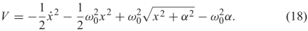
Subsequently,we apply the Theorem 1 and consider the Lyapunov function V（x）,as define by

We defin a set U={x∈Dr|V（x）≥0},where Dr= x∈R2|dist（x,ε1）≤risanenvironmentofε1andchoose r＞0,such that ε1?Dris the largest stationary set in Dr, as shown in Fig.5.

According to the properties of function V,we can fin that Vε=V（xm1）（or V（xm2））,where xm1（or xm2）∈bdry ε1（boundary of ε1）,xm1=（xm1,0）,xm2=（xm2,0）,and moreover,for?x0∈（xm1?δ,xm1）or x0∈（xm2,xm2+δ）, where δ＞0 is arbitrarily small,such that V（x0）＞Vε＞0, where x0=（x0,0）.Thus,the preconditions the Theorem 1 are satisfie and?σV＞0,such that V（x0）=Vε+σV.

The time-derivative of V obeys

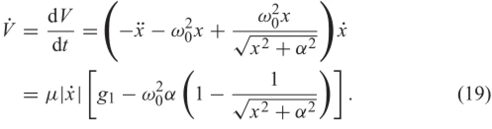
Looking at the condition（8）,it is noted that˙V≥0 for all （x,）∈U and˙V=0 if and only if˙x=0.Defin

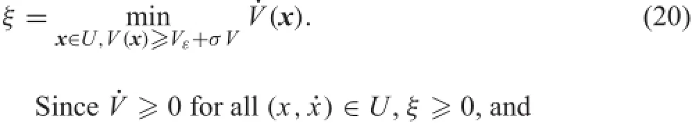
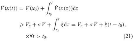
which excludes the possibility of solutions x（t）of the system（6）ultimately converging to ε1.Since U∩ε2=φ,ε1is the largest stationary set in Dr,we can easily know that the solutions of the system（6）can not stay in γε1,with γ={（x,˙x）|˙x=0}and γ?U,by using the equation of motion for system（6）.Thus,?t＞t0,such that x（t）/∈γ, moreover,everysolutionsofsystem（6）iscontinuousintime and x（t）/∈γ for a small time interval（t0,t1）.Therefore,we have that˙V＞0 for t∈（t0,t1）,which implies that V（t）is increasing for t∈（t0,t1）.As t→+∞,the solution will be bounded away from the equilibrium set ε1for an initial condition arbitrarily close to this equilibrium set.It can be concluded that the equilibrium set ε1is unstable.

4.2Stability of equilibrium sets ε2

In order to consider the stability property of the equilibrium sets ε2（ε2rand ε2l）,the following theorem can be found in Ref.［11］and applied to prove asymptotic convergence of the sets ε2,if the trajectories of non-smooth systems in Filippov-type are unique in forward time.

Theorem 2（stabilitytheoremforequilibriumsets（LaSalle’s invariance principle））

Let ε be an equilibrium set of the differential inclusion,

Let V（x）:Rn→R be a continuously differentiable and positive definit function,and suppose thatis bounded and that˙V≤0 for all x∈Ωl.Defin

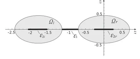
Fig.6　SchematicrepresentationofthesetΩr（showningrey）inwhich V≥0（V as in Eq.（23））

If ε be the largest invariant set in ξ,then the equilibrium set ε is locally attractive.

Firstly,we consider the stability of the right equilibrium set ε2rby using the Theorem 2.

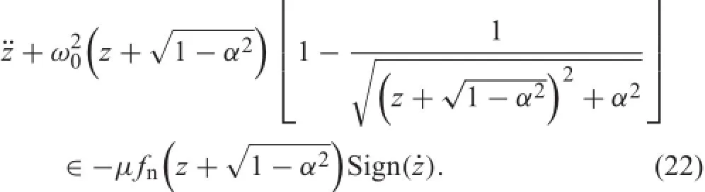
Byletting z=x?,thesystem（6）takestheform We apply the Theorem 2 and check the conditions stated therein.

The Lyapunov function V is chosen as following

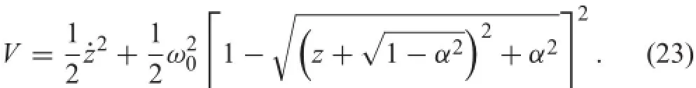
It is noted that V is a positive definit function since V＞ 0 for all（z,）∈Ωrε2rwithand V（0）=0,as shown in Fig.6.

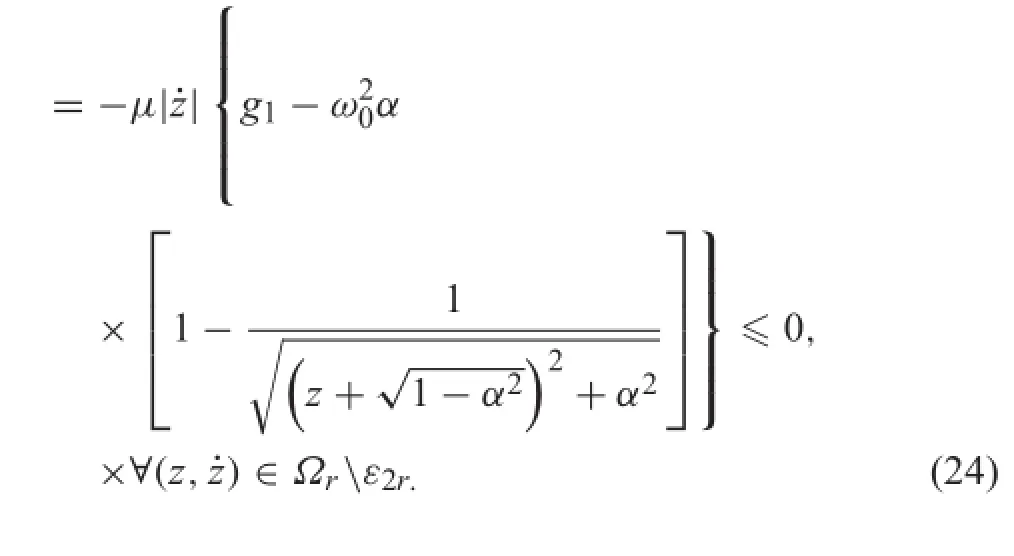
From the Eq.（8）,the time-derivative of V reads

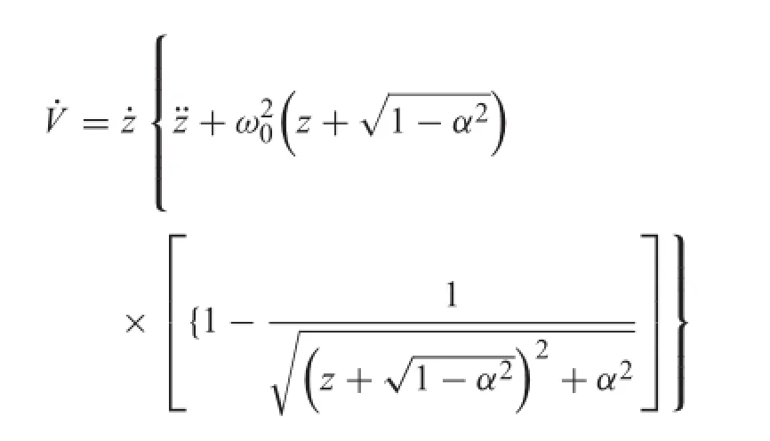
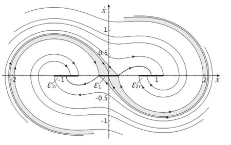
Fig.7　Phase plane of the SD oscillator with dry friction for α=0.4, g1=2,ω0=1,μ=0.1.The unstable equilibrium set ε1has a stable manifold（depicted in grey）,the unstable manifolds of ε1originate at the tips of the set ε1and are heteroclinic orbits to the stable equilibrium set ε2

It is realized that˙V=0 on the set Γ define by Γ=（z,）∈R2|=0and.

For the problem under consideration,the invariance principle can be applied since the trajectories are unique in forward time for this Filippov-type system.It is shown that the equilibrium set ε2ris the largest invariant set in Γ,then it is locally attractive.The equilibrium set ε2lcan also be proved to be attractive by applying the Theorem 2 in the set Ωl,due to the symmetry of the equilibrium sets ε2rand ε2r.

The phase plane of the SD oscillator with dry friction is showninFig.7fortheparameterα=0.4,whereequilibrium set ε1becomes a saddle point for μ=0,and the ε1becomes a set instead of a point when μ＞0,but the saddle structure in the phase plane remains.Interestingly,the unstable equilibrium set ε1has a“thick”stable manifold depicted in grey inFig.7,whereabundleofsolutionsexistandbeattractedto the unstable equilibrium set ε1.Furthermore,this phenomenon once appeared in Ref.［18］,and it will be discussed in the next section.The unstable manifolds of the set ε1originate at the tips of the set ε1and are heteroclinic orbits to the stable equilibrium set ε2.It is noticed that a equilibrium set of the system,which exhibits a stable equilibrium without dry friction,will be attractive with dry friction added. Moreover,a unstable equilibrium for the system without dry frictionwillbechangedintoaunstableequilibriumsetunder friction conditions,and itself is stable.

Fig.8 Phase plane of the SD oscillator with dry friction for g1=2,ω0=1,μ=0.1.a α=0.b α=1

With the different values of parameter α,we can get the stability property of all the equilibrium sets in this system by using the same methods above.Figure 8a shows the phase plane of the SD oscillator with dry friction for α=0.It is found that two table equilibria in the SD oscillator without friction become both two table equilibrium sets（ε3land ε3r）when the dry friction be added,but the point（0,0）（marked by a small red cycle in Fig.8a）not be changed,and the structurenearthispointstilllookslikeasaddlebehavior［20］. When α=1,the SD oscillator without friction has only one equilibriumpoint（0,0）,andthispointwillbechangedintoa equilibriumsetwithfrictionadded.Thissituationisdepicted in Fig.8b,where only one stable equilibrium set ε4exists.

5　Filippov’s property

Inorder toinvestigate theinteriorstabilityofthe equilibrium set,the concept of Filippov’s sliding mode is employed,see Refs.［16,24］.Three domains are distinguished on the discontinuity surface Σ,which is define by a smooth scalar function ?（x）.If the trajectories on both sides arrive at the boundary,then an attracting sliding mode occurs,where the domain is labeled as the sliding region Σs.If one side of the boundaryhastrajectoriestowardstheboundary,andtrajectories on the other side leave the boundary,then this domain is calledthecrossingregionΣc.Otherwise,theunstablesliding motion occurs on the domain Σu.The mentioned domains are identifie as follows and shown schematically in Fig.9.

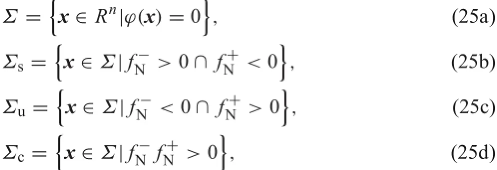
In this system,since ?（x）=˙x and x∈R2,we have

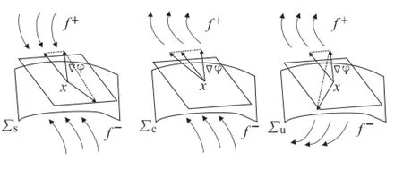
Fig.9 Discontinuity surfaces Σs,Σc,Σuof sets（25）in Filippov system

From the definition（25）mentioned above,we can obtain that

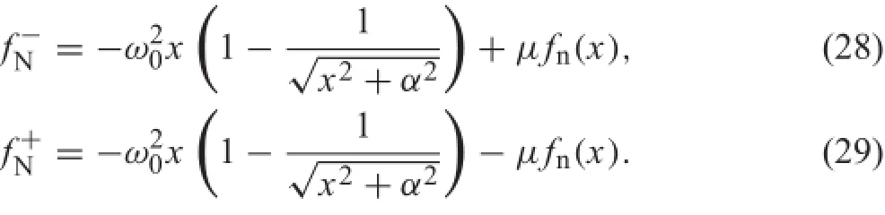
Figure 10 represents the attractive sliding regions Σs（marked as heavy lines）and crossing regions Σc（marked as dashed lines）on the discontinuous surface Σ of the system （6）,andnounstableslidingregionexists.Fromthedefinitio （25b）and Fig.10,we know that trajectories of the system （6）on both sides of the sliding region are directed to the equilibrium set εi（i=1,2）,and the interior points of theequilibrium set are stable since the attracting sliding mode occurs.

Fig.10 Stable sliding regions Σs（x∈Σ and f?N＞0∩f+N＜0）and crossing regions Σc（x∈Σ and f?Nf+N＞0）of the system（6）for parameter μ=0.1,g1=2,ω0=1,α=0.4

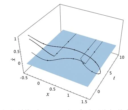
Fig.11 Sticking phenomenon on the surface˙x=0（depicted in dark）of the system（6）

In Fig.11,the trajectories of the system（6）slide along thesurface˙x=0 wherestickingoccurs.Whenthishappens, sliding along the surface˙x=0 in the t-direction of the phase space（x,˙x,t）,meaning that the mass sticks to the surface˙x=0.It is noted that the sliding here corresponds to the mechanical sticking［26］where˙x=0,as opposed to slipping where˙x/=0.Note that this leads to an unavoidable linguisticambiguity:physicallythemassstickstotheground, yet mathematically it is said to be sliding.So that the sliding region in this system is also called a stick region,which is fille with infinit equilibrium points.

A equilibrium set εiis divided into interior points Iiand two endpoints Eias follows:

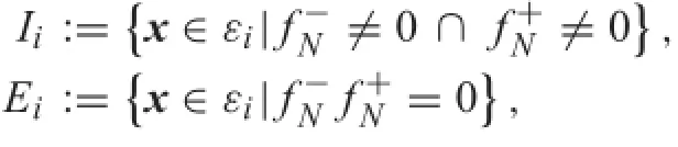
We defin that:

i=1,2,which determines the linearized dynamics near the endpoints of the equilibrium set.By calculating the eigenvalues of the Jacobian matrix near the endpoints,we fin that the endpoints（xm1,0）and（xm2,0）of the equilibrium set ε1are saddle-saddle points［15］,so the equilibrium set ε1is also called a hyperbolic equilibrium set.The endpoints （xr1,0）and（xr2,0）of the equilibrium set ε2rare focusfocus points［15］,so are the endpoints（xl1,0）and（xl2,0）of the equilibrium set ε2l,and the equilibrium sets ε2rand ε2lboth are called non-hyperbolic equilibrium sets.It has been shown that stability of the endpoints of the equilibrium set are the same as the stability of the whole equilibrium set.

6　Bifurcation of the equilibrium

Since the SD oscillator without dry friction is an archetype oscillator,which behaves with smooth and discontinuous propertiesaccordingtothesmoothparameterα,thepresence of dry friction can affect the dynamic behaviour of the SD oscillator.Especially,thestictionphenomenoninfrictioncan induce the presence of the equilibrium set,which can affect the whole dynamics of the SD oscillator.In order to examine the influenc of the parameter α and friction coefficien μ on the SD oscillator,we investigated the bifurcations of the equilibriumsetsinthesystem（6）,assuming g1=2,ω0=1.

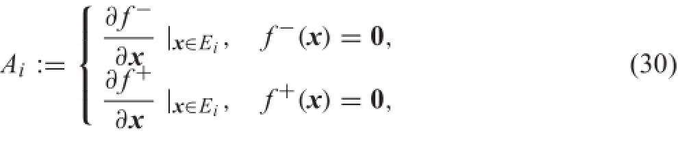
Figure 12a shows the body of the equilibrium sets ε for the system（6）in（x,α,μ）space,which is divided into four domains ofA,B,C,andD bytheplanesα=1 andμ=0.5. The bifurcation of equilibrium of SD oscillator without dry friction（μ=0）is shown in Fig.12b,where a pitchfork bifurcation happens at α=1.In Fig.12c,there are two stable equilibrium sets and a unstable equilibrium set merging into one large stable equilibrium set as α increases from 0 to 2 for friction coefficien 0＜μ＜0.5 in A-B domains. When μ≥0.5,the system（6）has only one equilibrium set with the change of α from 0 to 2 in C-D domains, as shown in Fig.12d.The SD oscillator is a discontinuous system,which has two stable equilibria,and a unstable saddle-like point when α=0,but when friction is added, it has two equilibrium sets and a saddle-like point,which merge into one large equilibrium set as μ increases from 0 to 1 in Fig.12e.In Fig.12f,when 0＜α＜1,there are two stable equilibrium sets and one unstable equilibrium set in the system（6）merging into one stable equilibrium set with the increasing of μ from 0 to 1 in A-D domains. Fig.12g shows that the system（6）has only one equilibrium set as μ increases from 0 to 1 in B-C domains whenα≥1.

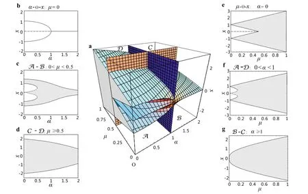
Fig.12　Bifurcationsoftheequilibriumsetsofthesystem（6）.a Bodyoftheequilibriumsetsin（x,α,μ）spaceisdividedintofourdomainsmarked byA,B,C,andDby the planes α=1 and μ=0.5.b μ=0 in α-x plane;c 0＜μ＜0.5 inA-Bdomains.d μ≥0.5 inC-Ddomains.e α=0 in μ-x plane.f 0＜α＜1 inA-Ddomains.g α≥1 inB-Cdomains

In Fig.12b-g,the points of the solid and dashed curves representthestableandunstableendpointsintheequilibrium sets,respectively,andthepointsoftheareainlightgreycolor represent the inner points of the equilibrium sets.

In order to demonstrate the rich dynamics of the SD oscillator with dry friction,the ridge and valley curves of the equilibria body can be exhibited by projecting the surface onto the parametric（α,μ）plane.The bifurcation branch of the equilibria marked as H1is obtained,where curve

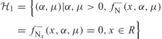
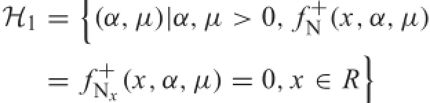
divides the parametric（α,μ）plane into two distinct regions marked by I,II,as shown in Fig.13Π.

In Fig.13,the phase portraits of this system for parameters all over the regions are also plotted.The bifurcation diagram Fig.13Π shows the transitions from multiple equilibrium sets merging into one stable equilibrium set in phase portraits.The discontinuous（α=0）phase portraits of SD oscillator with dry friction are presented to show the nonsmooth dynamic behaviors,marked as H2and C1,where the point C1denotes the transition from a saddle-like point （markedbyaredsmallcycle）andtwostableequilibriumsets in picture marked with H2merging into one stable equilibriumset.Whenα＞0,thephaseportraitsoftheSDoscillator with dry friction are shown in pictures marked as I,H1and II,where the curve H1presents the transition from three equilibrium sets merging into one equilibrium set,as shown in corresponding pictures from I to II.The dynamic behaviors of the SD oscillator without dry friction（μ=0）in discontinuous and smooth stages are marked as C3,H3,C2, respectively.

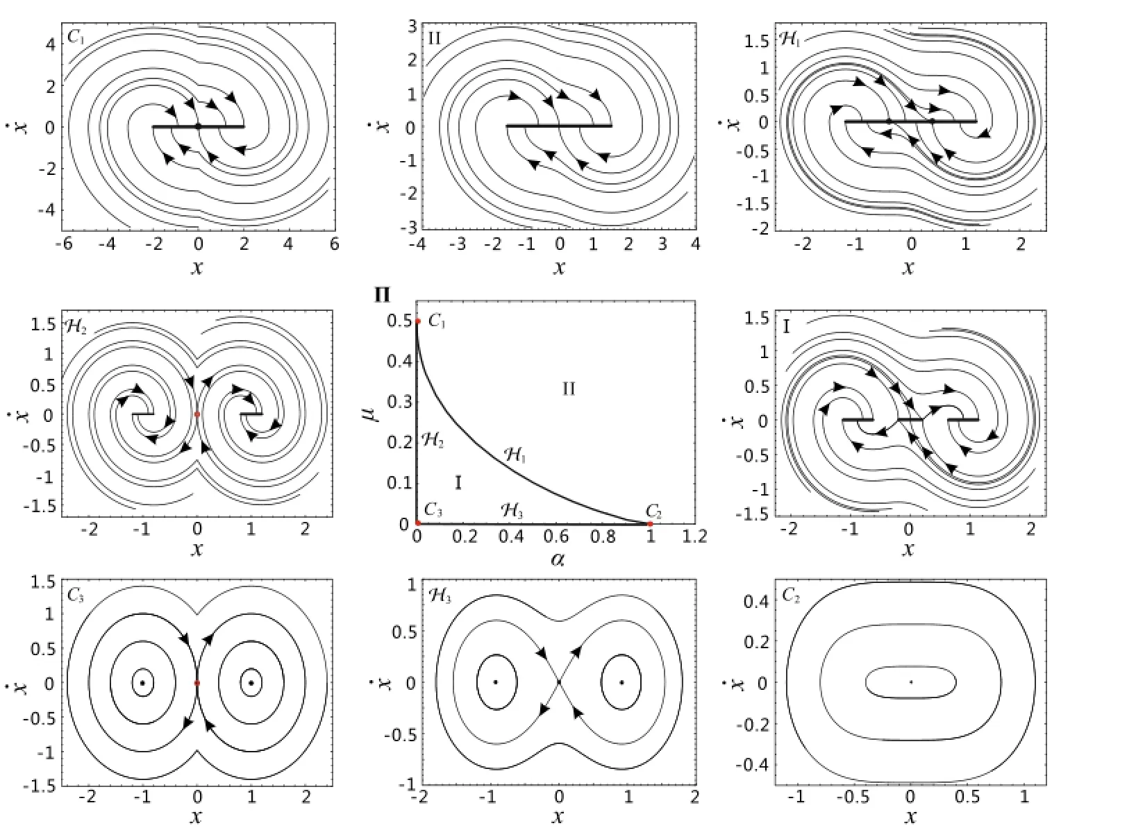
Fig.13　Bifurcation diagram and phase portraits of the system（6）.The transition branchH1divides the parametric（α,μ）plane into two distinct regions,marked as I,II,respectively,in which the corresponding phase portraitsH2and I for multiple equilibrium sets,C1andH1for transitions from multiple equilibrium sets merging into one equilibrium set,II for one equilibrium set,while C2,H3,C3for frictionless

7 Conclusions

In this paper we have focussed our attention on the equilibrium stability of the recently proposed SD oscillator with dry friction,which is a Filippov system with multiple stick regions.We have presented the sets of equilibrium states of this system in both（fn,fs）and（x,˙x）planes with the help of Coulomb’s cone for different values of parameter α. Lyapunov functions are constructed to get the global instability of the hyperbolic equilibrium set and the stability of non-hyperbolic type by using Lasalle’s invariance principle. It has been shown that the attractive sliding mode of this Filippov system generates the property that the hyperbolic equilibrium set has a thick stable manifold,and their interior points are stable.Furthermore,the unstable manifolds of the hyperbolic equilibrium set originate from the endpointswiththeirsaddleproperty.Duetothestabilityanalysis of the equilibrium set,all the stable and unstable ones for this system have been classifie and their bifurcations have also been displayed in smooth and discontinuous regimes. Phase portraits have also been plotted to demonstrate the complex transitions from multiple equilibrium sets to one equilibrium set for this non-smooth system with irrational nonlinearity. AcknowledgmentsThe project was supported by the National Natural Science Foundation of China（Grant 11372082）and the National Basic Research Program of China（Grant 2015CB057405）.

References

1.Shaw,S.W.:Onthedynamicresponseofasystemwithdryfriction. J.Sound Vib.108,305-325（1986）

2.Liu,X.J.,Wang,D.J.,Chen,Y.S.:Self-excited vibration of the shell-liquid coupled system induced by dry friction.Acta Mech. Sin.11,373-382（1995）

3.Elmer,F.J.:Nonlinear dynamics of dry friction.J.Phys.A 30, 6057-6063（1997）

4.Lamarque,C.H.,Bastien,J.:Numericalstudyofaforcedpendulum with friction.Nonlinear Dyn.23,335-352（2000）

5.Cheng,G.,Zu,J.W.:Dynamics of a dry friction under two frequency excitations.J.Sound Vib.275,591-603（2004）

6.Wiercigroch,M.,Pavlovskaia,E.:Engineeringapplicationsofnonsmooth dynamics.Nonlinear Dyn.Phenom.Mech.SMIA 181, 211-273（2012）

7.Luo,A.C.J.,Gegg,B.C.:Periodic motions in a periodically forced oscillator moving on an oscillating belt with dry friction.ASME J. Commun.Nonlinear Dyn.1,212-220（2006）

8.Leine,R.I.,VanCampen,D.H.,DeKraker,A.:Stick-slipvibrations induced by alternate friction models.Nonlinear Dyn.16,41-54 （1998）

9.Ding,W.J.,Fan,S.C.,Lu,M.W.:A new criterion for occurrence of stick-slipmotionindrivemechanism.ActaMech.Sin.16,273-281 （2000）

10.van de Wouw,N.,van den Heuvel,M.N.,Nijmeijer,H.:Performanceofanautomaticballbalancerwithdryfriction.Int.J.Bifurc. Chaos 15,65-82（2005）

11.Leine,R.I.,van de Wouw,N.:Stability and Convergence of Mechanical Systems with Unilateral Constraints.Lecture Notes in Applied and Computational Mechanics,vol.36.Springer,Berlin （2008）

12.Shevitz,D.,Paden,B.:Lyapunov stability theory of nonsmooth systems.IEEE Trans.Autom.Control 39,1910-1914（1994）

13.Bacciotti,A.,Ceragioli,F.:Stabilityandstabilizationofdiscontinuous systems and nonsmooth lyapupnov functions.ESIAM Control Optim.Calc.Var.4,361-376（1999）

14.Basseville,S.,Léger,A.,Pratt,E.:Investigation of the equilibrium states and their stability for a simple model with unilateral contact and Coulomb friction.Arch.Appl.Mech.73,409-420（2003）

15.Benjamin,Biemond:J.J.,vandeWouw,N.,Nijmeijer,H.:Bifurcations of equilibrium sets in mechanical systems with dry friction. Physica D 241,1882-1894（2012）

16.Filippov,A.F.:Differential Equations with Discontinuous Righthand Sides.Kluwer Acadamic,Dordrecht（1988）

17.Yakubovich,V.A.,Leonov,G.A.,Gelig,AKh:Stability of Stationary Sets in Control Systems with Discontinuous Nonlinearities. World Scientific Singapore（2004）

18.Leine,R.I.,van de Wouw,N.:Stability properties of equilibrium sets of nonlinear mechanical systems with dry friction and impact. Nonlinear Dyn.51,551-583（2008）

19.Cao,Q.J.,Wiercigroch,M.,Pavlovskaia,E.E.,et al.:Archetypal oscillator for smooth and discontinuous dynamics.Phys.Rev.E. 74,046218（2006）

20.Cao,Q.J.,Wiercigroch,M.,Pavlovskaia,E.E.,etal.:Thelimitcase response of the archetypal oscillator for smooth and discontinuous dynamics.Int.J.Nonlinear Mech.43,462-473（2008）

21.Cao,Q.J.,Wercigroch,M.,Pavlovskaia,E.E.,et al.:Piecewise linear approach to an archetypal oscillator for smooth and discontinuous dynamics.Philos.Trans.R.Soc.A 366,635-652（2008）

22.Tian,R.L.,Wu,Q.L.,Yang,X.W.,et al.:Chaotic threshold for the smooth-and-discontinuous oscillator under constant excitations. Eur.Phys.J.Plus 128,1-12（2013）

23.Léger,A.,Pratt,E.,Cao,Q.J.:A fully nonlinear oscillator with contact and friction.Nonlinear Dyn.70,511-522（2012）

24.Dieci,L.,Lopez,L.:Slidingmotioninfilipp vdifferentialsystems: theoretical results and a computational approach.SIAM J.Numer. Anal.47,2023-2051（2009）

25.Léger,A.,Pratt,E.:On the periodic solutions of a non smooth dynamical system.Rev.de Méca.Appli.et Théor.2,501-513 （2011）

26.Colombo,A.,Di Bernardo,M.,Hogan,S.J.,et al.:Bifurcations of piecewise smooth flws:perspectives,methodologies and open problems.Physica D 241,1845-1860（2012）

27.DiBernardo,M.,Budd,C.J.,Champneys,A.R.,etal.:Bifurcations in nonsmooth dynamical systems.SIAM Rev.50,629-701（2008）

12 January 2015/Revised:25 March 2015/Accepted:22 April 2015/Published online:6 September 2015

?Qing-Jie Cao

qingjiecao@hotmail.com

1School of Astronautics,Centre for Nonlinear Dynamics Research,Harbin Institute of Technology,Harbin 150001, China

2Laboratoire de Mécanique et d’Acoustique,CNRS,31, Chemin Joseph Aiguier,13402 Marseille Cedex 20,France