
A Third Derivative Estimate for Monge-Ampere Equations with Conic Singularities
2017-07-02 07:19:20GangTIAN
Gang TIAN
(Dedicated to Haim Brezis on the occasion of his 70th birthday)
1 Introduction
In this note,we extend a third derivative estimate in[4]to Monge-Ampere equations in the conic case.For the purpose of our application,we will consider the complex Monge-Ampere equations in this note.The same result holds for real Monge-Ampere equations.
Let U be a neighborhood of(0,···,0),and u satisfy

and

whereβ∈(0,1)andωβis the standard conic flat metric on Cn:

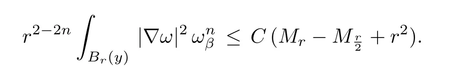
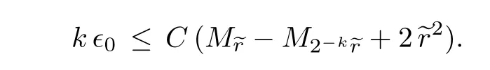
Theorem 1.1Let V be an open neighborhood of(0,···,0),whose closure is contained in U.Then for any α where Br(x)denotes the ball with center x and radius r,? is the covariant derivative,? denotes the Laplacian and the norm is taken with respect to ωβ. It follows from Theorem 1.1 and the standard arguments,e.g.,by using the Green function. Corollary 1.1Let u and F be as in Theorem 1.1.Then for any α ∈ (0,β?1? 1)and α<1,is Cα-bounded with respect to ωβ. This corollary was used by Jeffres-Mazzeo-Rubinstein in their proving the existence of K?hler-Einstein metrics with conic singularities.We refer the readers to Appendix B of[3]for details. Theorem 1.1 has been known to me for some time.The proof is identical to that in[4].Its arguments were inspired by Giaquinta-Giusti’s work(see[2])on harmonic maps.For years,I had talked about this approach to the C2,α-estimate for complex Monge-Ampere equations in my courses on K?hler-Einstein metrics. In this section,we prove Theorem 1.1 by following the arguments in Section 2 of[4].I will present the proof for complex Monge-Ampere equations in details.In[4],the proof was written for real Monge-Ampere equations,though it also applies to complex Monge-Ampere equations. Without loss of generality,we may assume x∈V∩{z1=0}.In fact,one can apply known estimates(see,e.g.,[4])to u outside the singular set{z1=0}ofωβ.If F is smooth on U,we can also apply Calabi’s third derivative estimate to u outside{z1=0}(see[5]). Define Bβ(r)to be the domain in C × Cn?1consisting of all(w1,w′),where w′=(w2,···,wn),satisfying There is an r>0 such thatand w′=(z2,···,zn)defines a natural map frominto U.This map is isometric from the interior ofonto its image.For convenience,we will use w1,···,wnas coordinates.By scaling,we may assume thatr=1. In terms of coordinates w1,···,wn,we have and covariant derivatives of u become ordinary derivatives,e.g., We will denote det(ukl)uijby Uij,where(uij)denotes the inverse of First we recall two elementary facts. Lemma 2.1(see[4,Lemma 2.1])For each j,where all derivatives are covariant with respect to ωβ. ProofRecall the identities Differentiating them in wk-direction and summing over k,we get Then the lemma follows. Lemma 2.2(see[4,Lemma 2.2])For any positive λ1,···,λn,we have where λ = λ1···λn,and C is a constant depending only on λiand ProofIn[4],(2.2)is proved by the properties of determinants.Here we outline a simpler proof.First by using the homogeneity and positivity of,we only need to prove the case whenNext,if we denote the left-hand side of(2.2)by f(Λ),then by a direct computation,for i=1,···,n.Then(2.2)follows from the Taylor expansion of f at I. In terms of w1,···,wn,(1.1)becomes By a direct computation,we deduce from this This system resembles the one for harmonic maps whose regularity theory were studied extensively in 70s and 80s.The idea of[4]is to apply the arguments,particularly in[2],from the regularity theory for harmonic maps. The following lemma follows easily from the Sobolev embedding theorem. Lemma 2.3There is a constant Cβ,which depends on β,such that for any smooth function h on Bβ=Bβ(1)with boundary condition we have Note that Cβblows up whenβtends to 1. Lemma 2.4(see[4,Lemma 2.3])There is some q>2,which may depend on β,and,such that for any,we have whereand C denotes a uniform constant.1Note that C,c always denote uniform constant though their actual values may vary in different places. ProofFirst we assume y=x.Defineλijby By using unitary transformations if necessary,wemay assumefor anyand i,j ≥ 2.It follows from(1.2)that where I denotes the identity matrix. Choose a cut-off function η:Br(x)7→ R satisfying Using Lemma 2.1 and(2.4),we can deduce whereand λ = λ1···λn. Using Lemma 2.1,we have Then by Lemma 2.2,we can deduce from the above that By applying the Sobolev inequality to(i,j ≥ 2)and Lemma 2.3 toin the above,we get This inequality still holds,if we replace Br(x)by any Br(y)which is disjoint from the singular set{z1=0}.This can be proved by using the same arguments,but Lemma 2.3 is not needed.One can easily deduce from this and a covering argument that for any ball B2r(y)?U, Then(2.7)follows from Gehring’s inverse H?lder inequality(see[1]). Lemma 2.5(see[4,Lemma 2.4])For any y∈V and B4r(y)?U andσ Multiplying(2.10)bywe get It follows that Multiplying(2.4)by b w and integrating by parts,we have Using the assumption that?F is bounded,we can easily deduce from this By Lemma 2.4 and the Poincare inequality,we have Without loss of generality,we may assume that q≥2(q?2).Sincevanishes on?Br(y),its L2-norm is controlled by the L2-norm ofand consequently,of|?ω|.Then we have Next,we recall a simple lemma which can be proved by standard methods. Lemma 2.6Let h be any harmonic function on Bβ=Bβ(1),such that Then for any r<1, In fact,we only need a weaker version of Lemma 2.6 in the subsequent arguments:In addition to the assumption(2.15),we may further assume Remark 2.1If we replace(2.15)by then we have a better estimate We observe Hence,by(2.11)and(2.18),we get Clearly,(2.9)follows from(2.12)–(2.14)and(2.19). In view of(2.9),we need the following lemma. Lemma 2.7(see[4,Lemma 2.5])For any ?0>0,there is an ?depending only on ?0,and inf?F satisfying that for any e r>0 with Ber(y)? U,there issuch that ProofIt follows from(2.4)that where?′denotes the Laplacian ofω. Letηbe a non-negative function on Br(y)satisfying thatη(z)=1 for anyη(z)=0 for any z near ?Br(y)andThen where SetIt follows from(2.21)that for a suitable constanti.e.,Z is super-harmonic with respect toω.Sinceω is equivalent toωβ,we can apply the standard Moser iteration to?′to get It follows that Hence,if(2.20)does not hold forthen This is impossible if k is sufficiently large.So the lemma is proved. Now we complete the proof of Theorem 1.1.Chooseξ=λ2αandλ∈(0,1),such that Next we choose?0and r0sufficiently small,such that Then we can deduce from(2.9)that forσ=λr and r≤r0satisfying(2.20), whereν = β?1?1>α.Then(1.3)follows again from this and a standard iteration. [1]Gehring,W.,The Lp-integrability of the partial derivatives of a quasiconformal mapping,Acta Math.,130,1973,265–277. [2]Giaquinta,M.and Giusti,E.,Nonlinear elliptic systems with quadratic growth,Manuscripta Math.,24(3),1978,323–349. [3]Jeff res,T.,Mazzeo,R.and Rubinstein,Y.,K?hler-Einstein metrics with edge singularities(with an appendix by C.Li and Y.Rubinstein),Annals of Math.,183,2016,95–176. [4]Tian,G.,On the existence of solutions of a class of Monge-Ampere equations,Acta Mathematica Sinica,4(3),1988,250–265. [5]Yau,S.T.,On the Ricci curvature of a compact K?hler manifold and the complex Monge-Ampere equation,I,Comm.Pure Appl.Math.,31,1978,339–411.
2 The Proof of Theorem 1.1


 Chinese Annals of Mathematics,Series B2017年2期