Faculty of Electrical Engineering,Mathematics and Computer Science,Delft University of Technology,Mekelweg 4,2628 CD Delft,The Netherlands

E-mail: N.Huang-1@tudelft.nl

Yutao MA (馬宇韜)?

School of Mathematical Sciences &Laboratory of Mathematics and Complex Systems of Ministry of Education,Beijing Normal University,Beijing 100875,China

E-mail: mayt@bnu.edu.cn

Abstract We use tridiagonal models to study the limiting behavior of β-Laguerre and β-Jacobi ensembles,focusing on the limiting behavior of the extremal eigenvalues and the central limit theorem for the two ensembles.For the central limit theorem of β-Laguerre ensembles,we follow the idea in [1] while giving a modified version for the generalized case.Then we use the total variation distance between the two sorts of ensembles to obtain the limiting behavior of β-Jacobi ensembles.

Key words beta-ensembles;largest and smallest eigenvalues;central limit theorem;total variation distance

1 Introduction

Aβ-Laguerre ensemble,also called a Wishart ensemble,is a set of non-negative random variables λ :=(λ1,λ2,···,λn) with the joint density function

Aβ-Jacobi ensemble,also called theβ-MANOVA ensemble,is a set of random variables μ :=(μ1,μ2,···,μn) ∈[0,1]nwith a joint probability density function

In 2002,Dumitriu and Edelman proved that theβ-Laguerre ensembles can be seen as the eigenvalues of real symmetric tridiagonal random matrices,which are distributed asin Table 1 ([3]).The calculations in this note are all based on the tridiagonal model.In fact,in the same paper,Dumitriu and Eldeman also gave the random tridiagonal model of another sort ofβ-ensemble,theβ-Hermite ensemble,which we are not going to discuss here.The tridiagonal model of theβ-Jacobi ensembles was achieved in [7] and [10].Jiang ([9]),Ma and Shen ([12])used the tridiagonal model to calculate the distances between the two sorts of ensembles;this is quite useful in terms of understanding the limiting behavior ofβ-Jacobi ensembles through theβ-Laguerre ensembles.

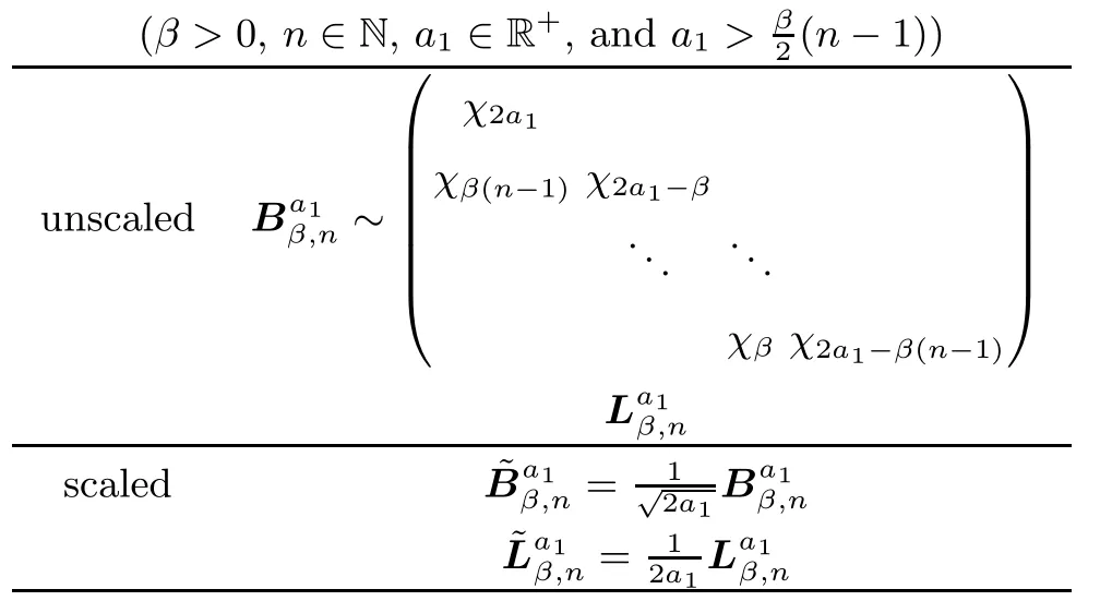
Table 1 Unscaled and scaled tridiagonal models for beta-Laguerre ensembles

Based on the tridiagonal random matrices,Dumitriu and Edelman gave the central limit theorem for theβ-Laguerre ensembles in [2].Let (λ1,λ2,···,λn) be the beta-Laguerre ensembles of parametera1and sizen,whose joint density function is given by (1.1).Assume that,and let.For anyi≥1,let

Setλmax=max{λ1,λ2,···,λn},λmin=min{λ1,λ2,···,λn} and assume that(0,1].Then

almost surely.This result was first reported without proof in [1],and then in [9],the proof was given by Jiang.

Let (μ1,μ2,···,μn) be random variables with density functionfβ,a1,a2,defined in (1.2).In [9],Jiang obtained similar results for extremal eigenvalues and the central limit theorem for empirical measures.Settingμmax=max{μ1,μ2,···,μn},μmin=min{μ1,μ2,···,μn},and assuming that,we then have that in probability asn→+∞.

Given any integeri≥1,define

fori≥1.Similarly,assume thatand that,(X1,···,Xk) converges weakly to a multivariate normal distribution for anyk≥1.

A considerable amount of literature has been devoted to the eigenvalue distributions of beta ensembles.Dumitriu and Koev presented explicit formulas for the distributions of the extreme eigenvalues of theβ-Jacobi random matrix ensemble in terms of the hypergeometric function of a matrix argument (see [3]),and Edelman and Koev presented the explicit expressions forβ-Laguerre ensembles (see [4]).Dumitriu and Paquette studied global fluctuations for linear statistics of theβ-Jacobi ensembles (see [5]).It is also worth mentioning that Killip studied the Jacobi ensembles and proved Gaussian fluctuations for the number of points in one or more intervals in the macroscopic scaling limit given in [6].Trinh in [14] gave a unified way to offer the central limit theorems via spectral measures for beta ensembles and also investigated the Gaussian fluctuation around the limit.

Recently,high-dimensional data has appeared in many fields,and analysis of this data has become increasingly important in modern statistics.However,it has long been observed that several well-known methods in multivariate analysis become inefficient,or even misleading,when the data dimensionp,which is equivalent to the parameter 2a1/βin this note,is much larger than the sample sizen.Here a high dimensional scenarion/p→0 is considered.

1.1 Main results for β-Laguerre ensembles

The main results forβ-Laguerre ensembles in this note are as follows:

Theorem 1.1Let (λ1,λ2,···,λn) be theβ-Laguerre ensembles of parametera1and size n,whose joint density function is given by (1.1).Assume that.Then asn→∞,

almost surely.

In particular,forγ=0,almost surely for all 1 ≤i≤n.

The following theorem is an extension of Theorem 1.5 in [2]:

Theorem 1.2Let (λ1,λ2,···,λn) andγbe defined as Theorem 1.1.For anyk≥1,set

where(t) is defined as in (1.3).Then,for any integerm≥1,asn→∞,

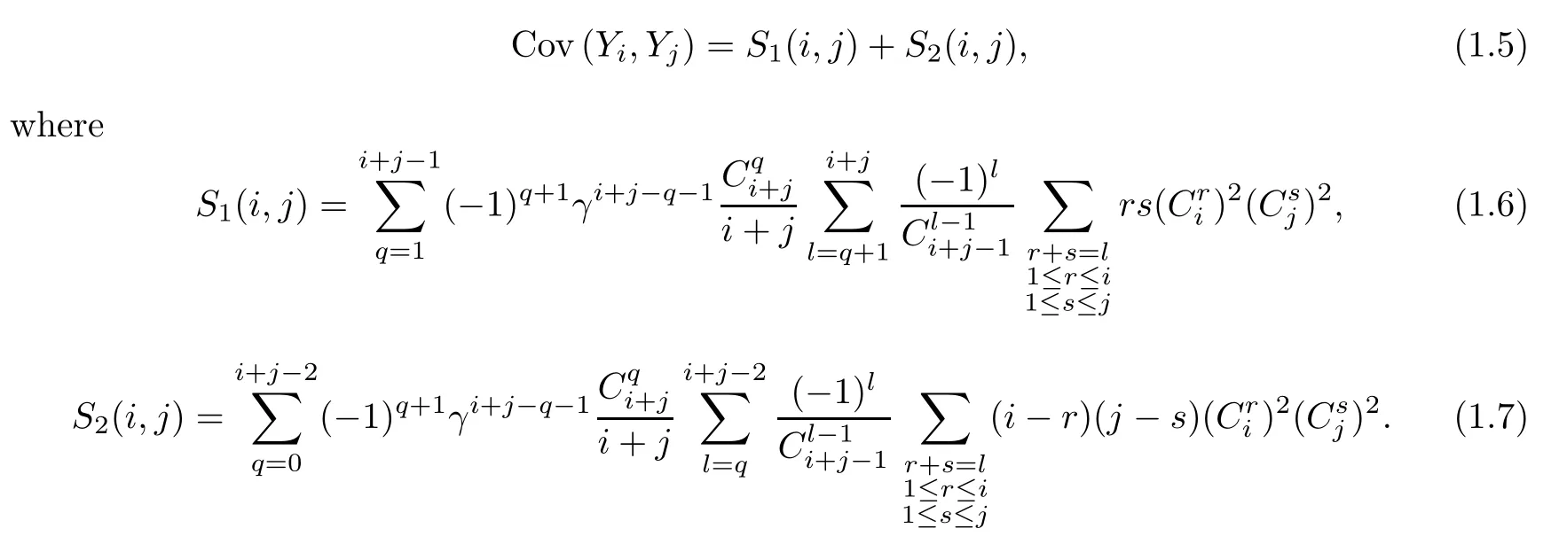
Here (Y1,Y2,···,Ym) is a centered multivariate Guassian with the covariance matrix

Remark 1.3There is an inconsistency in Theorem 1.5 in [2],which we found is established only for,but not for the genereal case.Take the following case as an example:

Suppose that (λ1,λ2···,λn) are the eigenvalues ofthen

Taking scaling into account,we have that

According to the central limit theorem from Dumitriu (Theorem 1.5 in [2]),

wherecis a constant;this contradicts (1.8),therefore,we need to make a slight modification and rewrite the formula as (1.4).

Remark 1.4It is easy to see that whenγ=0,

Therefore,for ?i,j≥1,

The improvement from the result of Dumitriu and Edelman in [2] is reflected in the power ofγin (1.6) and (1.7).In [2],the central limit theorem is only adaptable for 0＜γ≤1.Here,we obtain a more general consequence adaptable for 0 ≤γ≤1.

1.2 Main results for β-Jacobi ensembles

For Jacobi ensembles,we utilize the conclusions ofβ-Laguerre to yield the relative results ofβ-Jacobi through the connection between the two ensembles.The following lemma was first proved by Jiang in [9] for,and then generalized by Ma and Shen in[12] fora1n=o(a2) :

Lemma 1.5Let λ=(λ1,λ2,···,λn) and let μ=(μ1,μ2,···,μn) be the random variables with density functions (1.1) and (1.2),respectively.Denote with ||L(2(a1+a2)μ)-L(λ)||the total variation distance between the probability distributions of 2(a1+a2)μ and λ.Assume thata1n=o(a2).Then

Following the method in [9],and based on Lemma 1.5 and Theorem 1.1,we can easily have

Theorem 1.6Let (μ1,μ2···,μn) be theβ-Jacobi ensembles with density functionfβ,a1,a2given by (1.2).Recall thatμmax=max{μ1,μ2,···,μn},μmin=min{μ1,μ2,···,μn}.Suppose thata1n=o(a2) and

in probability.

Similarly,utilizing Lemma 1.5 and Theorem 1.2,we have

Theorem 1.7Define

Suppose thata1n=o(a2).Then for any givenm≥1,

where (Y1,Y2,···,Ym) is the same as in Theorem 1.2.

2 The Proof of Theorem 1.1: the Extremal Eigenvalues for β-Laguerre Ensembles

We can see a set of random variables from theβ-Laguerre ensembles as the eigenvalues of the corresponding tridiagonal model,which is,where

Lemma 2.1

forj=2,···,n.Note thatis a tridiagonal symmetric matrix.

In this section,we will prove the limiting behaviour of the extremal eigenvalues ofThe idea is borrowed from [13] (Silverstein 1985).To prove Theorem 1.1,we first introduce two lemmas.

Lemma 2.2χnis a chi distribution with n degrees of freedom,soalmost surely asn→∞.

ProofAscan be seen as the sum of the squares ofnindependent normal random variables,according to Kolmogorov strong law of large numbers,we have that

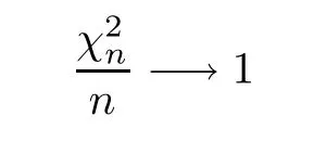
almost surely asn→∞.Note that the property of convergence is maintained under the transformation of continuous functions,thus

almost surely asn→∞. □

The proof of Theorem 1.1From Theorem 6.0.5 in [1],we know that

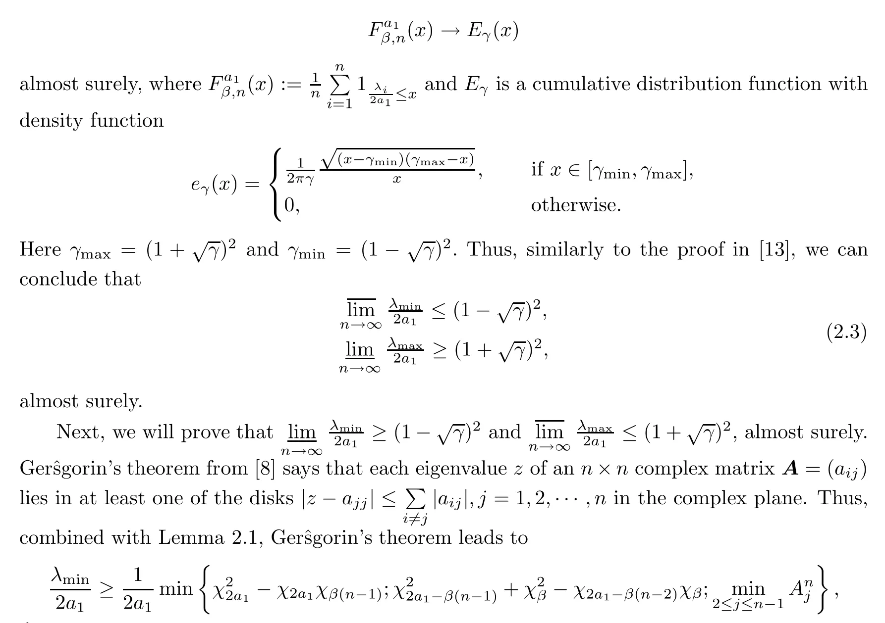
almost surely asn→∞,and

Combining (2.3) and (2.4),we conclude that

almost surely.In a similar way,we have that

almost surely. □

3 The Proof of Theorem 1.2: CLT for β-Laguerre Ensembles

In this section,we are going to prove Theorem 1.2.The proof is divided into two parts.

Lemma 3.1(the fluctuation) Recall,fork≥1,that

where (Y1,Y2,···,Ym) is a centered multivariate Guassian defined as in Theorem 1.2.

Lemma 3.2(The deviation) With the same assumption as in Lemma 3.1,fornlarge enough,we have that

where(t) is as defined by (1.3).

Remark 3.3In particular,ifγ=0,

fornlarge enough.

3.1 The proof of Lemma 3.1: the fluctuation

To prove Lemma 3.1,we are going to prove the following claims first (all the notations are defined as above):

Claim 1Setfor anyk≥1.For any positive integerskandl,

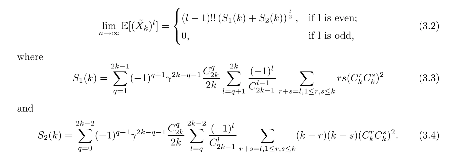
Claim 2For any fixed positive integersiandj,

whereS1(i,j),S2(i,j) are defined as in (1.6) and (1.7).

Claim 3For any(1 ≤ki≤n),and ?ti∈R(i=1,···,m),

The proof of the three claims are basically the same,and the idea also comes from [2].Before the proof,we first introduce some notations.

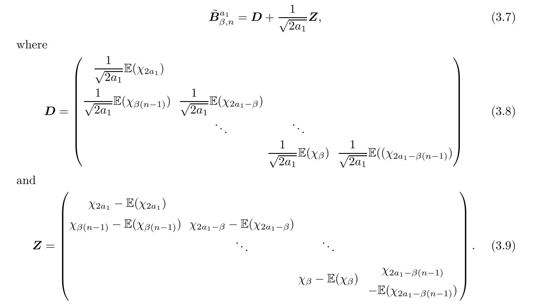
Remark 3.4As in [2],the entries ofDare bounded and for any finitekandlthere exists a constantMsuch that

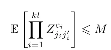
for all 0 ≤ci≤kland for allj1,···,jklandsuch that

For the expression of tr((BBT)k),it holds that

where the sum is taken over sequences (i1,···,i2k) with the property thati2j-1-i2j∈{0,1}(for all 1≤j≤k),i2j-i2j+1∈{0,-1} (for all 1 ≤j≤k-1),and alsoi2k-i1∈{0,-1}.

Definition 3.5Denote bySn,k∈{1,···,n}2kthe set of sequences of integersi1,···,i2ksuch thati2j-1-i2j∈{0,1} for all 1≤j≤k,andi2j-i2j+1∈{0,-1} for all 1 ≤j≤k-1,and alsoi2k-i1∈{0,-1}.

We allow for the possibility of having empty sequencesip0,···,ip1in the beginning and/orip2q,···,ip2q+1in the end ofJ.

Definition 3.6For any I ∈,we introduce the set J=J (I) of pairs (J,R) corresponding to the sequence I.For a bidiagonal matrixB,donote that B*=BTifij-ij+1=-1,otherwise,B*=B.Define

Remark 3.7Note that any term in trwill consist of terms in D and terms in Z,with a sequence of runsJrecording the former,and a sequence of runsRrecording the latter.

The proof of Claim 1For simplicity,setAccording to the definition above,we have that

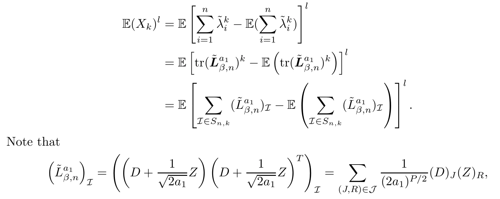
withP=p2-p1+1 +···+p2q-p2q-1+1.Thus,

In the next lemma,we will present some results from [2] which also hold here.

Lemma 3.8Assume that (R1,R2,···,Rl) involves s independent variables.The only terms of asymptotical significance are those for whichs=q=l/2;this means that forkandlfixed,iflis odd,

Therefore,we only need to examine what happens whenlis even ands=q=l/2.

Lemma 3.9Iflis even,s=q=l/2,and we have |Rj|=1.This means that for each 1 ≤j1≤l,there exists a unique 1 ≤j2≤lsuch thatZRj1=ZRj2.Moreover,given an orderedl/2-tuplet of distinct indicesi1,i2,···,il/2,there are (l-1)!! ways of pairing these indices to thein this order.

The next two lemmas are about the estimation of (Z)Rjand (D)Jj;there are slight differences from [2].Also we only need to consider the significant terms.

Lemma 3.10For (ZRj) we have that

Lemma 3.11For (D)Jj,assuming that IJjhave 2soffdiagonal terms,there are two cases:

1) when (Z)Rjcorresponds to a diagonal term,then there exists anisuch that (Z)Rj=Ziiand there are 2(k-s)()2corresponding to IJj,and

2) when (Z)Rjcorresponds to an offdiagonal term,then there exists anisuch that (Z)Rj=Zi+1,i,and there are 2s()2corresponding to IJj,and

The proof of Lemmas 3.10 and 3.11By Lemma 7.1.2 in [1],we know that if∞,then

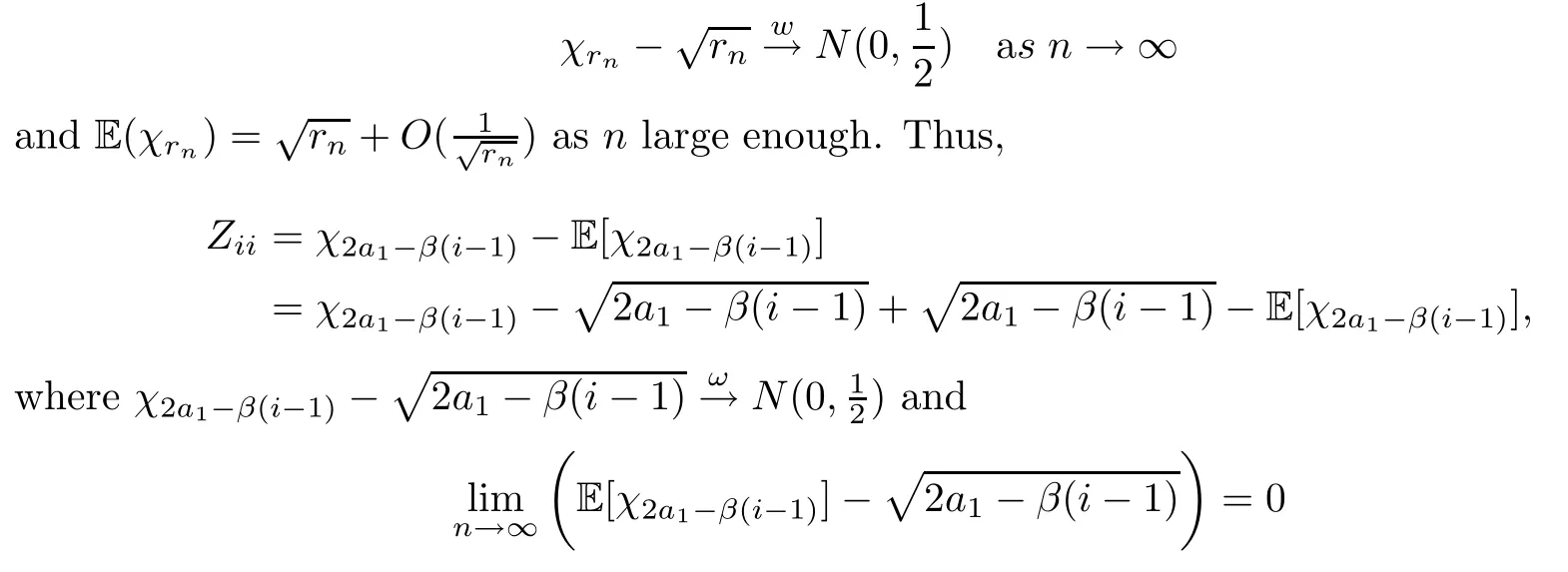
for anyisatisfyingi＜＜a1.Therefore,(3.12) is established.

In the same way,we know that for the entries ofD,asnis large enough,we have that

for anyisatisfyingi＜＜a1.Therefore,(3.13) and (3.14) hold. □

Combining the above lemmas,iflis even,we can easily obtain equation:

First,calculateS1,n.For simplicity,set

By binomial expansion and a changing summation order,we have that

Using the properties of the Riemann integral and the Beta function,we know that

Hence,plugging (3.17) into (3.16),we have that

Therefore,Claim 1 is established. □

The proof of Claim 2For anyk1,k2≥1,by the precedent calculations,we have that

whereqis the total length ofR1andR2.The contribution terms are for |R1|=|R2|=1 andR1=R2.Similarly,we have that

Repeating a process similar to that of Claim 1,we obtain the equation (3.5).This means that Claim 2 is established. □

The proof of Claim 3For simplicity,we takem=2,for example.For otherm≥1,the process is basically the same.In fact,for anyt1,t2∈R andk1,k2≥1,we have that

wherepis the number of pickingk1among the product oflterms,andqis still the total length ofRj.

By Lemmas 3.8,3.9 and 3.10,iflis odd,it holds that

In the next calculations,we only need to consider what happens whenlis even.The only difference from the proof of Claim 1 is in terms of the estimation of (D)Jj.

Now,we can obtain the estimation of (D)Jjunder the three combinations.Note that for combination (k1,k2),there are two choices for the correspondingR.Thus,we have the following formula:

Obviously,it holds that

whereS1,n(ki,kj) andS2,n(ki,kj)(i=1,2) are defined as in (3.18);S1(ki,kj) andS2(ki,kj)(i=1,2) are defined as in (1.6) and (1.7).Putting (3.20) back into (3.19),for evenl,we have that

Setm≥1.For anyti∈R and any integerki≥1,the following conclusion can be obtained similarly:

Lemma 3.1 follows directly from Claim 1,Claim 2 and Claim 3.

3.2 The proof of Lemma 3.2: the deviation

In this section,we are going to prove Lemma 3.2.

The proof of Lemma 3.2According to Chapter 6.3 in [1],if 0＜γ≤1,fornlarge enough,we have that

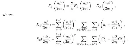
for anyk≥1,whereis a polynomial ofwith respect tok.More precisely,

and AGDk,rdenotes the set of alternating Motzkin paths of length 2kwithrrises,ui(p) denotes the number of rises between altitutesiandi+1 in pathpandli(p) denotes the number of level stepsptaken from altitudeion odd-numbered steps.

Through the proof of Lemma 2.20 in [2],when

Combining (3.21) and (3.22),since,it is easy to find out,that fornlarge enough,

Therefore,returning to (3.21),

Naturally,if 0＜γ≤1,(3.23) yields the following result:

By definition,ui(p)=0 for anyp∈AGDk,0and anyi≥1.This means,for the casefornlarge enough.Therefore,

fornlarge enough.The proof is now complete. □