Numerical study of the flow in the Yellow River with non-monotonous banks*
He-fang JING (景何仿), Yi-tian LI (李義天), Chun-guang LI (李春光)
?
Numerical study of the flow in the Yellow River with non-monotonous banks*
He-fang JING (景何仿)1,2, Yi-tian LI (李義天)2, Chun-guang LI (李春光)1
1. State Key Laboratory of Water Resources and Hydropower Engineering Sciences, Wuhan University, Wuhan 430072, China 2. Research Institute of Numerical Computation and Engineering Applications, North University for Nationalities, Yinchuan 750021, China, E-mail: jinghef@163.com (Received April 6, 2014, Revised May 27, 2014)
A 2-D depth averaged RNGmodel is developed to simulate the flow in a typical reach of the Upper Yellow River with non-monotonic banks. In order to take account of the effect of the secondary flow in a bend, the momentum equations are modified by adding an additional source term. A comparison between the numerical simulation and the field measurements indicates that the improved 2-D depth averaged RNGmodel can improve the accuracy of the numerical simulation. An arc spline interpolation method is developed to interpolate the non-monotonic river banks. The method can also be reasonably applied for the 2-D interpolation of the river bed level. Through a comparison of the water surface gradients simulated in the seven bends of the studied reach, some analytical formulae are improved to reasonably calculate the longitudinal and transverse gradients in meandering river reaches. Furthermore, the positions of the maximum water depth and the maximum velocity in a typical bend are discussed.
2-D RNGmodel, numerical simulation, extra source term, arc cubic spline interpolation, non-monotonic bank
Introduction
The flow structures in rivers with bends are very important in river engineering as they are closely rela- ted to the river flooding prediction, the bank prote- ction, the water intakes, the navigation, and the evolu- tion of the river-bed and the sediment transport. As al- most all natural rivers are meandering, the study of the flow structures in meandering rivers/channels is of enormous practical importance in engineering applica- tions. Therefore, in past decades, the flow structures in meandering rivers/channels were extensively studied using various approaches, such as the theoretical ana- lysis, the laboratory experiments and the numerical si- mulation.
In a theoretical analysis, some theoretical solutio- ns or empirical formulae are developed to calculate the flow structure in meandering rivers/channels[1]. However, they more often than not contain some sim- plifications of the flow conditions, and some are obtai- ned by analyzing the measured data. Therefore, they may not be valid for all flow conditions. The labora- tory experiment is a very important approach to study the flow structures in meandering rivers[2,3]. However, expensive economical and time investments are invo- lved. With the development of the computational me- thods and computer techniques, numerical simulations are increasingly applied for the simulation of the flow in rivers and channels. In past decades, many methods were developed and used to simulate the turbulent flow in rivers or open channels, such as the methods based on the potential flow theory[4], the direct nume- rical simulation (DNS)[5], the large eddy simulation (LES)[6,7], and the Reynolds averaged numerical simu- lation (RANS)[8,9]. Though the DNS and the LES are more accurate, their huge computation requirement li- mits their applications in the numerical simulation of natural rivers. Compared with the DNS and the LES, the RANS needs less computation time and is widely applied in numerical simulations of flows in rivers/ channels. For the RANS, we have the zero equation model, themodel, the Reynolds stress equation model (RSM), and the algebraic stress model (ASM), etc.[10,11]. Among these turbulent models, themodel is more adaptive than the zero equation model and it requires less computation time than the RSM and the ASM. As a result, it is widely used to numeri- cally simulate all kinds of flows, such as open channel flows, river flows and pipe flows[12,13]. However, the standardmodel may produce distorted results when it is used to simulate some complex flows, such as the flow with a high strain rate, and the flow with a large streamline curvature. For the flow with a high strain rate and a large streamline curvature, the renor- malization groupmodel (RNGmodel) is applied in order to obtain accurate simulation results.
The flow in meandering rivers is 3-D and should be simulated by 3-D turbulence models. However, because of the long computation time and the storage requirement for the computer, 3-D turbulence models are difficult to be applied to simulate the flow and the sediment transport in a long river reach for long time. Therefore, the depth-averaged and the 2-D depth ave- raged mathematical models were proposed. Generally speaking, 2-D models can not reflect the influence of the secondary flow in meandering rivers, and the simulated results are usually not satisfactory. In order to solve this problem, various schemes were proposed in recent years. Lien et al.[14]developed a 2-D model with consideration of the influence of the secondary flow through calculating the dispersion stress produ- ced by the discrepancy between the mean and the true velocity distributions. Kimura et al.[15]applied a 2-D depth averaged model to simulate the open channel flow in a side-cavity, in which the effects of the seco- ndary flow are integrated by adding an extra source term in the momentum equations. However, the above models can only be used in laboratory regular mean- dering channels. In the above models, the additional source terms in the momentum equations are very complicated, and the governing equations are usually formulated in orthogonal coordinates, in which the velocity components are not natural. In addition, most of these models use laminar flow models or zero equa- tion models. Therefore, they are not easy to be applied to numerically simulate the turbulent flow in meande- ring natural rivers.
In this study, a 2-D depth averaged RNGmodel is developed by averaging the 3-D RNGmodel in depth and by adding an extra source term of the momentum equations in the body-fitted coordinate system. The model is applied to simulate the turbulent flow in the Daliushu Reach of the Yellow River. Si- mulated velocity and water level agree well with the field measured data. The water surface slopes along the longitudinal and transverse directions in typical bends of the studied river reach are simulated and ana- lyzed. The distributions of the turbulence kinetic ene- rgy and the turbulence dissipation rate at some typical cross-sections are also discussed. Numerical examples indicate that the improved 2-D RNGmodel can reasonably simulate the turbulent flow in rivers with monotonic banks.
Before simulation, some preprocessing work is required, such as the river bank interpolation, the to- pography interpolation, and the mesh generation. Be- cause the boundary of the simulated physical area is non-monotonic, the most effective interpolation me- thod, i.e. the cubic spline interpolation, becomes inva- lid for the bank interpolation in the studied reach. In addition, the ordinary 2-D interpolation methods also do not work when they are used for the topography in- terpolation. In order to solve these problems, a new method based on the cubic spline interpolation, named as the arc cubic spline interpolation, is developed for the bank and topography interpolations in this study. Examples show that the arc cubic spline interpolation is very efficient when it is used for the non-monoto- nic river bank interpolation and the 2-D topography interpolation. The improved RNGmodel, inco- rporated with the sediment model, can also be applied to simulate the sediment transport and the bed defor- mation in rivers or open channels. The simulated resu- lts will be presented in subsequent papers.
1. Mathematical model
In a body-fitted coordinate (BFC) system, five governing equations of the 2-D RNGmodel can be written in the following universal form[16,17]
where

Table 1 The variables in the universal governing equation
In order to take account of the influence of the secondary flow in meandering rivers, the following extra source terms are added in the momentum equa- tions inanddirections, respectively[17]:
Generally speaking, the grid step in thedire- ction is far greater than that in thedirection. As a result,andcan be neglected comparing withand. So Eq.(2) can be rewritten as follows:
The additional source terms inanddirections can be obtained by combining the above equations.
Furthermore, supposing thatandare constant alongdirection, the above equations can be rewri- tten as follows:
After adding the additional source terms in the mo- mentum equations, the new source terms of the mo- mentum equations inanddirections become
It can be found that the additional source terms in the momentum equations inanddirections are mainly determined by the velocity, the water depth and the curvature radius of the bend. The absolute va- lues of the additional source terms increase with the increase of the bend curvature, the velocity of the flow, and the water depth. Generally speaking, the seconda- ry flow increases with the increase of the bend curva- ture, the flow velocity and the water depth. Further- more, the secondary flow increases with the increase of the transverse gradient of the longitudinal flow ve- locity and the water depth. So, the above additional source terms can reasonably reflect the effect of the secondary flow in meandering rivers.
2. Numerical methods
2.1
The finite volume method (FVM) is used to dis- cretize Eq.(1). The computational domain is rectangu- lar in the BFC system and can be easily divided into a series of small rectangles. A collocated grid system is adopted in this study. The momentum interpolation method is applied in order to avoid the checkerboard pressure difference[18], respectively. The east, west, south and north neighbor nodes ofare,,and, respectively, the second east, west, south and north neighbor nodes ofare,,,,respectively. Integrating Eq.(1) over the control volu- meyields
The first term (i.e. the unsteady term, represented by) on the left hand side is discretized by the first order implicit scheme. The second and third terms (i.e. the convective terms) on the left hand side are discre- tized using a modified QUICK scheme[19]. As a result, the scheme not only has the third order accuracy, but also is diagonally dominant, which can easily be sol- ved by the tri-diagonal matrix algorithm (TDMA)[10].
The first and second terms on the right hand side (i.e. the diffusion terms) are discretized using the se- cond order central difference scheme. The last term on the right hand side (the source term) can be dealt with by using the local linear method. The collocated grid SIMPLEC algorithm in the BFC system is used to solve the coupled problem of the water level and the velocities.
The discretized equations are solved by the itera- ted method. Within each time step (the inner iteration), the criterion of convergence is as follows
2.2
Before simulation, the position of the river banks is to be interpolated by the coordinates measured at the cross-sections, as shown by Fig.1. The linear inter- polation is one of the simplest interpolation methods. However, the banks obtained by the linear interpola- tion are not smooth. As a result, the numerical results obtained by using the linear interpolation are not relia- ble.
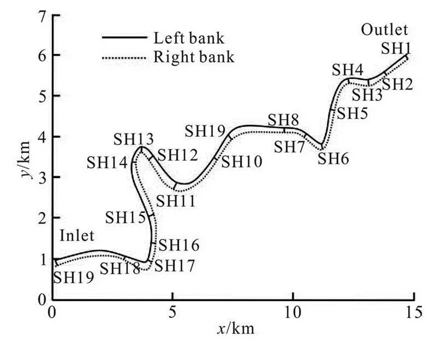
Fig.1 The plain view of Daliushu reach in the Yellow River
The cubic spline interpolation is one of the effe- ctive methods widely applied in engineering. However, when the method is applied to interpolate the studied river banks, the result is obviously not satisfactory, as shown in Fig.2. In fact, the method can only be used when a bank is monotonic. In other word, at least the horizontal coordinates or the longitudinal coordinates of the bank should be monotonic In order to satisfy the requirement, the studied banks are usually divided into several pieces and the cubic spline interpolation is applied at each piece. Though it is more reasonable to use the cubic spline interpolation and the results are smoother than by using the linear interpolation, the curve calculated by the method is still not smooth enough at the joint of two pieces. In addition, the bank must be divided into several pieces based on monoto- nous requirements, which is time consuming and di- fficult to operate.
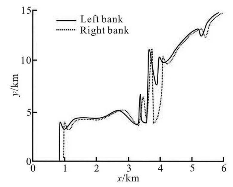
Fig.2 Banks calculated by cubic spline interpolation
In this study, the arc cubic spline interpolation is developed, which is not only easy to operate, but also more accurate or more reasonable than the linear in- terpolation, the cubic spline interpolation and the pie- cewise cubic spline interpolation. Letare the selected points on the curve of a bank, and they are arranged in sequential order.is the starting point, andis the end point. Letre- presents the arc length fromto, then the coo- rdinates
2.3
After the mesh generation, the next difficult pro- blem that needs to be solved is the topography inter- polation. In other words, the bed levels of all grid poi- nts are interpolated from the field measured data at the cross-sections. A number of 2-D interpolation sche- mes can be used, such the 2-D linear interpolation, the 2-D cubic spline interpolation, etc.. However, all these 2-D interpolation schemes require both the coordina- tesandof the studied area be monotonic. Ob- viously, as shown in Fig.1, the coordinatesandof the studied area are not monotonic. As a result, these schemes can not be used in this study. In order to solve this problem, two schemes are considered.
The first scheme is to transform the studied reach into a rectangle area using the BFC transformation. In the computational area, both the horizontal and longi- tudinal coordinates are monotonic, so we can use above 2-D interpolation schemes to obtain the bed level at the every mesh grids. We name the scheme as the 2-D inversion interpolation method. However, this scheme may bring about errors, especially when the mesh of the physical area is not divided equally. Ge- nerally speaking, the mesh of the computational area is uniform, but the mesh of the physical area is not. So the scheme is not suitable in this study.
The second scheme is to use the 1-D interpola- tion twice to obtain the bed level at the mesh grids. For convenience, the lines of the cross-sections are often chosen as a part of the grid lines (lines), as shown by Fig.3. So the first step is to get the bed level at the grid nodes of the cross-sections using the arc cubic spline interpolation. The next step is to obtain the bed level of all grid nodes in the studied reach. As shown by Fig.3, eachline is a curve that is parallel to the river banks approximately. After the first step, the topography at a certain number of points in eachline is obtained. Then the bed level of each grid point in anline can be calculated with the arc cubic spline interpolation. We call this scheme as the descending dimension arc cubic spline interpolation (DDACSIP) method.
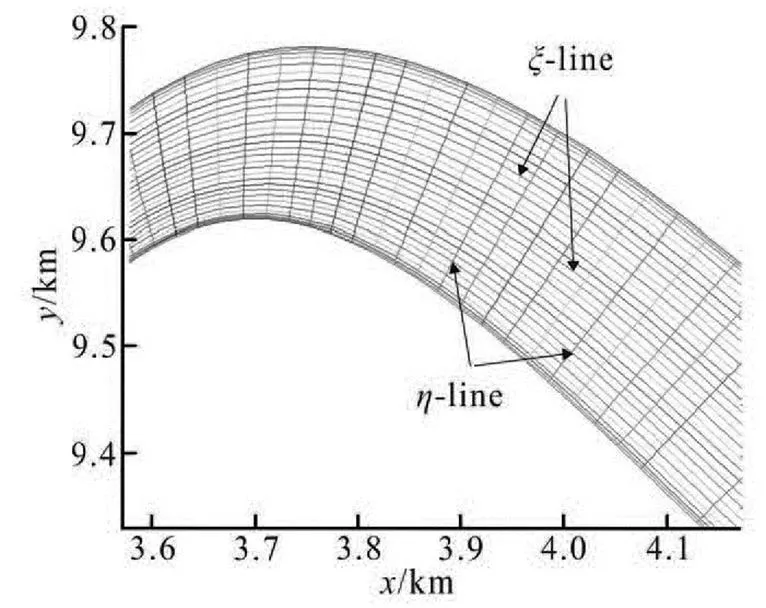
Fig.3 Local mesh of the studied river reach
Figure 4 shows the topography calculated by the DDACSIP method from the field measurement of the Daliushu Reach on 11-3-11-5, 2011. It can be found that the DDACSIP method is more reasonable and more accurate.
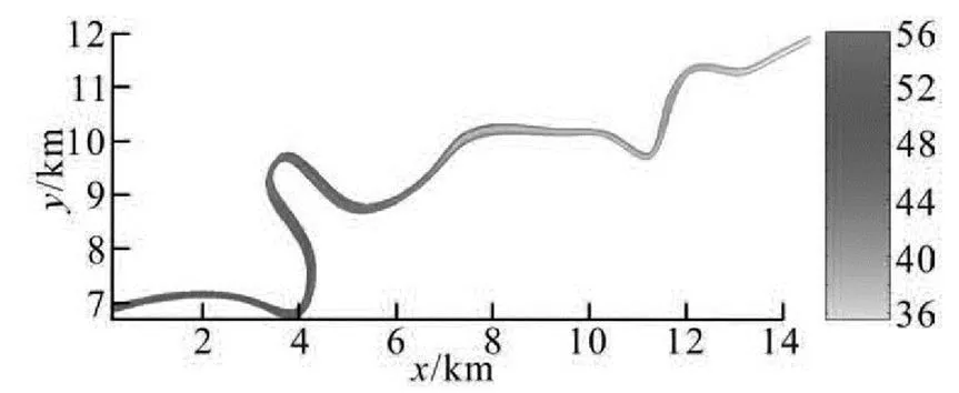
Fig.4 Bed level contour of the studied reach interpolated with DDACSIP method
2.4
On the water inlet, the depth averaged velocity magnitudeis given according to the field mea- sured data, and the velocity is perpendicular to the se- ction of the inlet. Its components inanddire- ctions (i.e.and) can be calculated by
The turbulence kinetic energy and its dissipation rate are calculated by the following formulae[20].
On the water outlet boundary, the water level needs to be set based on the measured data. Other va- riables, i.e.,,andare dealt with accordi- ng to the fully developed condition as follows
On the solid wall boundary (i.e. the river bank), in order to reduce the computation requirement, the wall function method[10]is adopted.andare set as zero at the grids on the banks, while,andare dealt with according to the symmetrical boundary as follows
2.5
The initial water level is linearly interpolated from the measured water level at the inlet and the out- let. The initial velocity componentsandat all nodes are set as zero except for those at the inlet. However, the initialandcan not be set as zero, asis the denominator of the source term in theequation. The improper initial value ofandwill lead to the interruption of the simulating process.
Two schemes can be used for setting the initial values ofand. The first scheme is to set the initial values ofandthe same as those at the inlet. Another scheme is to set the initial values ofandas fixed values, such as,,based on the experience of the authors.
3. Results and discussions
3.1
The studied reach, i.e. the Daliushu reach, is lo- cated at the later end of the Heishan gorge and it belo- ngs to the upper reach of the Yellow River. The total length of the Daliushu reach is 17.7 km, and the ave- raged width is only 155.2 m. The sinuosity of the stu- died reach is 0.887, and the total bed slope is equal to 0.09326%. On 11-3-11-5, 2010, 11-3-11-5, 2011 and 10-27-10-29, 2012, the research team of the authors went to the Daliushu Reach to make field measureme- nt for the velocity, the water depth, the water level and other basic data with instruments such as RiverCAT, GPS, etc..
The Daliushu Reach of the Yellow River consists of 7 bends, and 19 cross-sections are set up for measu- rement and analysis, as shown in Fig.1. These bends are irregular and there is no obvious straight part be- tween two adjacent bends. From the inlet to the outlet, these bends are Bend A (from SH19 to SH18), Bend B (from SH18 to SH15), Bend C (from SH15 to SH12), Bend D (from SH12 to SH10) and Bend E (from SH10 to SH7), Bend F (from SH7 to SH5), Bend G (from SH5 to outlet).
The river bed levels measured on 11-3-11-5, 2011 are used in the simulation. The discharge at the inlet is 1 110 m3/s, the averaged velocity is 1.64 m/s, the turbulence kinetic energy and the turbulence dissi- pation rate (and) at the inlet are calculated acco- rding to Eqs.(10a) and (10b), the water level at the outlet is equal to 1 242.4 m (the absolute value acco- rding to the Huanghai elevation system). The relative value of the water/bed level is calculated by subtra- cting 1 200 m from the absolute value of the water/ bed level. In this study, the relative water/bed level is adopted for convenience. The field measured bed level is shown in Fig.4. The difference between the water levels at the inlet and the outlet is about 16 m.
3.2
In the studied reach, along the longitudinal dire- ction (direction), 237 grid nodes are set, and along the transverse direction (direction), 31 grids are set. The total number of grid nodes and cells are 7 347 and 7 080, respectively. The Poisson equation method[10]is used to make the BFC transformation and the grid generation. The mesh density is set to be larger where the velocity gradient is larger, such as near the banks or near the apex of a bend. Figure 3 shows the mesh of Bend C in the studied reach.
3.3
In order to validate the mathematical model, four typical cross-sections (i.e. SH14, SH13, SH12, and SH11) are chosen to compare the depth averaged ve- locities measured and simulated with two different methods, as shown in Fig.5. In the first method (Me- thod 1), the numerical simulations are conducted using the 2-D RNGmodel without considering the effect of the secondary flow in a bend, while in the second method (Method 2), the numerical simulations are conducted using the improved 2-D RNGmodel that takes the effect of the circulation current into account. From Fig.5, it can be seen that Method 2 gives more accurate results than Method 1 by compa- ring the calculated velocities with the measured data on the four typical cross-sections.
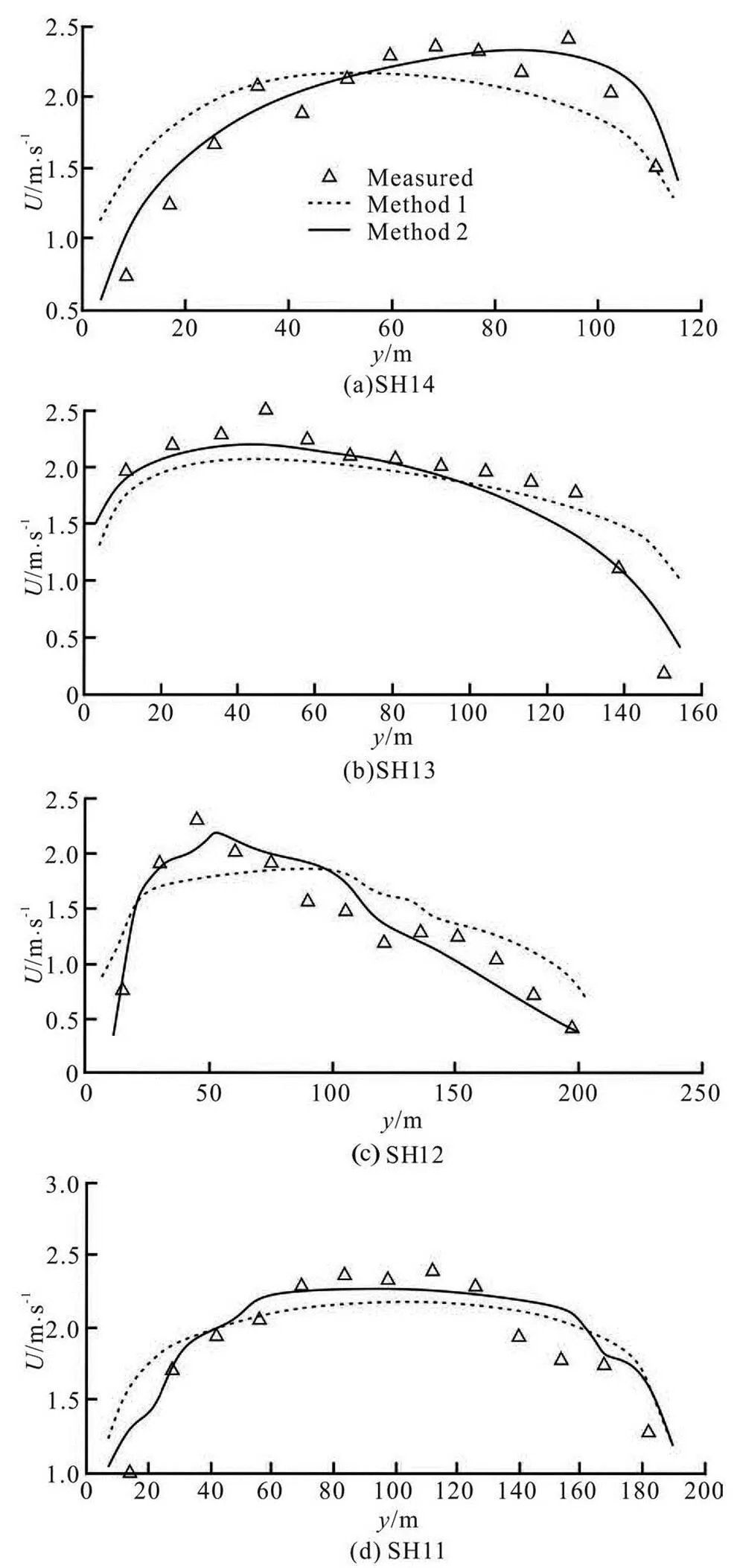
Fig.5 Comparison of velocities on typical cross-sections
The four cross-sections are located at Bend C in the studied reach, where the left bank is a concave bank, and the right bank is a convex bank. SH14 is at the inlet of Bend C, where the maximum velocity is found near the right bank (a convex bank). SH13 and SH12 are near the bend apex of Bend C, where the maximum velocity is found near the right bank (a con- cave bank). SH11 is at the outlet of Bend C, where the velocity is nearly uniform. So it can be concluded that both the measured and simulated velocities in Bend C are consistent with the basic rule of the bend flow, i.e. the maximum velocity is found near the convex bank at the inlet of a bend, then its position turns to the con- cave bank gradually and near the concave bank at the apex of the same bank, then it turns to the convex bank again, if the bend is fully developed, the velocity is nearly uniform at the outlet of the bend.
However, if we study the velocity distribution in other bends, the above rule does not seem always to hold. For example, SH11 is near the apex of Bend D, in which the left bank is a convex bank, while the right bank is a concave bank. But the maximum velo- city is not found close to the concave bank. The rea- son is that there is not an obviously straight transition section between Bend C and Bend D. In other words, the flow in bend C is not fully developed even after it reaches Bend D.
In general, the simulated values of the depth-ave- raged velocity agree well with the measured data on the four cross-sections, indicating that the improved 2-D RNGmodel can reasonably simulate the flow velocity in natural rivers with continuous bends.
3.4
Under the action of the centrifugal force in a bend, the water level near the convex bank will fall while the water level near the concave bank rises. As a result, the water surface along the transverse direction in a bend is not horizontal, and there is a transverse water surface slope in a bend.
The water levels on six typical cross-sections (From SH14-SH9) are presented in Fig.6. SH14, SH13 and SH12 are located at the inlet, the apex and the outlet of bend C, respectively, where the left bank is concave and the right bank is convex. We can see that the water level of the concave bank is higher than that of the convex bank on all these cross-sections. However, the transverse water surface gradients are different among these cross-sections. The transverse gradient of SH13 is the largest, the next is that of SH14 (0.058%), and the smallest is that of SH12. SH11 and SH10 are at the apex and the outlet of Bend D, respectively, where the left bank is convex and the right bank is concave. The water levels of the concave bank at SH11 and SH10 are higher than that of the convex bank. The water surface gradient is 0.024% at SH11, but it is only 0.0099% at SH10. SH9 is near the apex of Bend E. Similar to Bend C, the left bank is concave and the right bank is convex at Bend E, and the water surface level of the concave bank is higher than that of the convex bank.
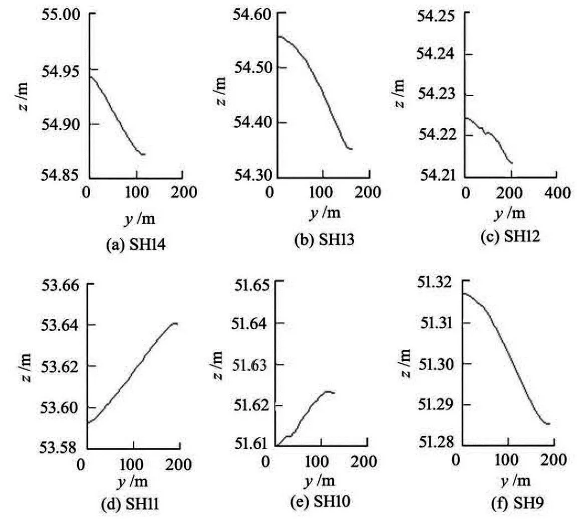
Fig.6 Comparison of water levels on some cross-sections
So it can be concluded that the water level of the flow in a continuous bend is consistent with the gene- ral rule of the bend, i.e. the water surface near the con- cave bank is higher than that near the convex bank, the transverse water surface gradient increases gradua- lly from the inlet to the apex of a bend, and then it de- creases gradually.
The transverse water surface gradient may be di- fferent in different bends. The transverse gradient of the water surface at the apex in a bend can be calcu- lated by the following formulae[21]:
Rosovsky formula
Makavejevsky formula
Zhang Hong-wu formula
From Eqs.(14)-(16), it can be seen that the tran- sverse gradient is proportional to the square of the averaged velocity and is inversely proportional to the curvature radius of the bend. However, as shown in Table 2, the transverse water surface gradients simula- ted at the apex of the bends in the studied river reach are not consistent with those calculated by Eqs.(14)- (16).

Table 2 Transverse gradient of water surface at the apex cross-sections in Daliushu Reach
Because Eqs.(14)-(16) are derived from regular curved channels or rivers, they are not suitable for ir- regular natural rivers with complicated topography. As the results calculated by above formulae are very similar, the Zhang Hong-wu formula can be improved as follows
The longitudinal water surface gradient in open channels can be calculated by the Chezy formula
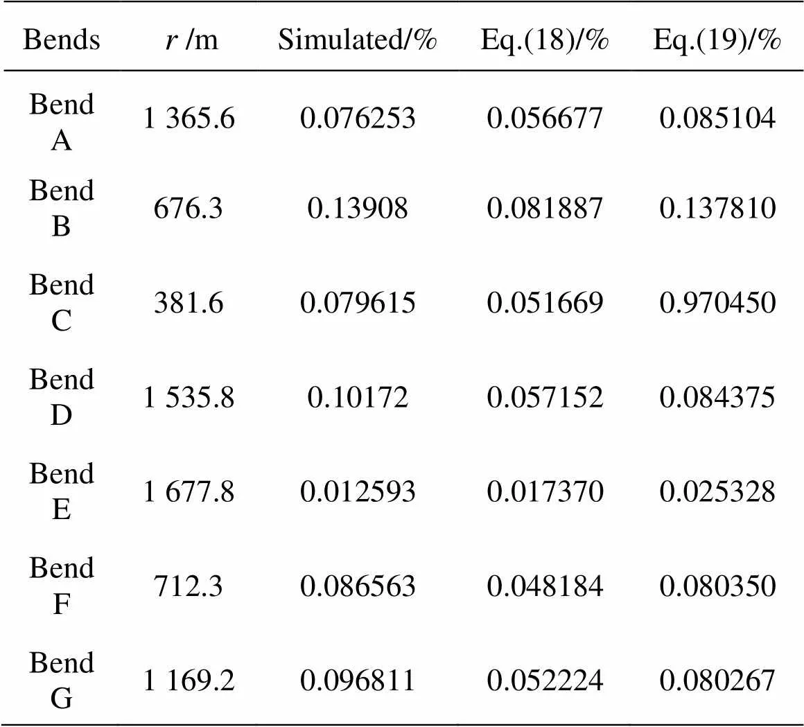
Table 3 Longitudinal gradient of water surface in bends of Daliushu Reach
Equation (18) is modified by adding an extra term as follows
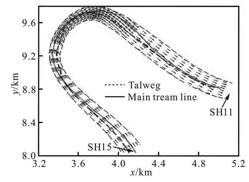
Fig.7 Simulated velocity field of the part from SH15 to SH11
From Eqs.(18) and (19), it can also be found that the increment of the longitudinal water surface gradie- nthas a close relationship with the radius of a bend. The increment will decrease with the increase of the radius of a bend, andif. As is known, the curved channel/river will tend to a straight one if its radius goes to infinity. So Eq.(19) can be regarded as the generalization of Eq.(18). Therefore, it can be used to calculate the lon- gitudinal water surface gradient of both straight and meandering channels/rivers.
3.5
Figure 7 shows the 2-D flow field of the part from SH15 to SH11 (which belongs to Bend C and Bend D). The positions of the talweg (where the water is the deepest along the river width) and of the main streamline (where the depth average velocity is the largest along the river width) are also plotted in Fig.7.
It is seen that the main stream is close to the con- vex bank at the inlet of the bend (SH15), and then it moves gradually to the concave bank. At the apex of the bend (SH13), the main stream is close to the con- cave bank. After that, it starts to move to the convex bank again. At the outlet of the bend (SH12), the main stream is at the position of the centerline of the bend. Then it moves to the concave bank of the next bend.
It can also be found that the talweg and the main stream line coincide at some parts of the domain inve- stigated, such as the position near the apex of the bend and the position near the outlet of the bend. In other word, the velocity is larger wherever the river is dee- per along the transverse direction in these positions. However, the talweg and the main stream line appear at different locations in the computational domain, such as the positions near SH15, SH14, and SH12. SH15 is at the junction of Bends B and C, and there is no obvious straight transition section between these bends. Near SH14, the river width is suddenly contra- cted. Near SH12, the river width is suddenly enlarged.
From the above analysis it can be concluded that the maximum water depth and the maximum velocity usually appear at different locations where the river width is suddenly contracted or suddenly enlarged, or at the junction of two different bends.
4. Conclusions
An arc cubic spline interpolation scheme is deve- loped for the bank and topography interpolations. Examples show that the scheme is very efficient when it is used for interpolations of river banks and 2-D to- pography when the river bank is non-monotonic.
The longitudinal and transverse water surface gradients are calculated and compared with some theoretical formulae. These theoretical formulae are improved according to the simulation results. Further- more, the positions of the talweg and the main stream- line are compared. They coincide at the some parts of the studied reach. However, at some positions, such as the junction of two bends and the positions where the river width is suddenly contracted or enlarged, they appear at different locations.
Acknowledgements
This work was supported by the Open Research Fund Program of the State Key Laboratory of Water Resources and Hydropower Engineering Sciences, Wuhan University (Grant No. 2013A011), the Foreign Expert Project of North University for Nationalities.
References
[1] PATRA K. C., KAR S. K. and BHATTACHARYA A. K. Flow and velcoity distribution in meandering compound channels[J]. Journal of Hydraulic Engineering, ASCE, 2004, 130(5): 398-411.
[2] CUI X., GRAY J. M. N. T. Gravity-driven granular free- surface flow around a circular cylinder[J]. Journal of Fluid Mechanics, 2013, 720: 314-337.
[3] WU Peng, HIRSHFIELD F. and SUI J. et al. Impacts of ice cover on local scour around semi-circular bridge abut- ment[J]. Journal of Hydrodynamics, 2014, 26(1): 10-18.
[4] GUO Y. Numerical modeling of free overfall[J]. Journal of Hydraulic Engineering, ASCE, 2014, 131(2): 134- 138.
[5] ROSTI M. E., CORTELEZZI L. and QUADRIO M. Dire- ct numerical simulation of turbulent channel flow over po- rous walls[J]. Journal of Fluid Mechanics, 2015, 784: 396-442.
[6] WANG J. K., MILANE R. E. Large eddy simulation (2D) of spatially developing mixing layer using vortex-in-cell for flow field and filtered probability density function for scalar field[J]. International Journal of Numerical Me- thods in Fluids, 2006, 50(1): 27-61.
[7] XIE Z., LIN B. and FALCONER R. A. Large-eddy simu- lation of the turbulent structure in compound open-channel flows[J]. Advances in Water Resources, 2013, 53(1): 66-75.
[8] JING H., LI C. and GUO Y. et al. Numerical simulation of turbulent flows in trapezoidal meandering compound open channels[J].International Journal of Numerical Metho- ds in Fluids, 2011, 65(9): 1071-1083.
[9] AMBROSINI W., PUCCIARELLI A. and BORRONI I. A methodology for including wall roughness effects inlow-Reynolds turbulence models, Part I. Basis of the methodology[J]. Nuclear Engineering and Design, 2015, 286: 175-194.
[10] VERSTEEG H. K., MALALASEKERA W. An introdu- ction to computational fluid dynamics, the finite volu- me method[M]Second Edition, London, UK: Pearson Education Limited, 2007.
[11] JING H., GUO Y. and LI C. et al. Three dimensional nu- merical simulation of compound meandering open channel flow by Reynolds stress equation model[J]. International Journal of Numerical Methods in Fluids, 2009, 59(8): 927-943.
[12] ZHENG J., MASE H. and DEMIRBILEK Z. et al. Imple- mentation and evaluation of alternative wave breaking for- mulas in a coastal spectral wave model[J].Ocean Engi- neering, 2008, 35(11-12): 1090-1101.
[13] GUO Y., ZHANG L. and SHEN Y. et al. Modelling study of free overfall in a rectangle channel with strip roughen- ss[J]. Journal of Hydraulic Engineering, ASCE, 2008, 134(5): 664-667.
[14] LIEN H. C., HSIEH T. Y. and YANG J. C. et al. Bend- flow simulation using 2D depth-averaged model[J]. Jour- nal of Hydraulic Engineering, ASCE, 1999, 125(10): 1097-1108.
[15] KIMURA I., ONDA S. and HOSODA T. et al. Computa- tions of suspended sediment transport in a shallow side- cavity using depth-averaged 2D models with effects of se- condary currents[J].Journal of Hydro-Environment Research, 2010, 4(2): 153-161.
[16] WU Xiu-guang, SHEN Yong-ming and ZHENG Yong- hong et al. 2-D flow SIMPLEC algorithm in non-orthogo- nal curvilinear coordinates[J].Journal of Hydraulic Engineering, 2003, (2): 25-30(in Chinese).
[17] JING H., LI C. and GUO Y. et al. Modelling of sediment transport and bed deformation in rivers with continuous bends[J]. Journal of Hydrology, 2013, 499(3): 224-235.
[18] CUBERO A., SANCHEZ-INSA A. and FUEYOA N. A consistent momentum interpolation method for steady and unsteady multiphase flows[J]. Computers and Chemical Engineering, 2014, 62(7): 96-107.
[19] HUA Zu-lin, XING Ling-hang and GU Li. Application of a modified quick scheme to depth-averagedturbule- nce model based on unstructured grids[J]. Journal of Hydrodynamics, 2008, 20(4): 514-523.
[20] KANG H., CHOI S. U. Reynolds stress modeling of re- ctangular open-channel flow[J]. International Journal of Numerical Methods in Fluids, 2006, 51(11): 1319-1334.
[21] XU Guang-xiang, TONG Si-chen and ZHONG Liang. Study on the longitudinal distribution of water surface transverse slope in curved conduits[J]. Journal of Hydro- electric Engineering, 2009, 8(4): 114-118(in Chinese).
* Project supported by the National Natural Science Foun- dation of China (Grant Nos. 91230111, 11361002), the Natural Science Foundation of Ningxia Hui Autonomous Region (Grant No. NZ13086).
Biography: He-fang JING (1970-), Male, Ph. D., Associate Professor
Corresponding author: Chun-guang LI, E-mail: cglizd@hotmail.com
10.1016/S1001-6058(15)60615-7 2016,28(1):142-152
- 水動力學研究與進展 B輯的其它文章
- Ski-jump trajectory based on take-off velocity*
- Formation of air-entraining vortices at horizontal intakes without approach flow induced circulation*
- Numerical simulation of flow and bed morphology in the case of dam break floods with vegetation effect*
- Numerical and experimental studies of hydraulic noise induced by surface dipole sources in a centrifugal pump*
- Pelton turbine: Identifying the optimum number of buckets using CFD*
- Mass transport in a thin layer of power-law fluid in an Eulerian coordinate system*

