Yanjun Guo ,Jiao Li,Jianping Xiong ,Jiangdan Li,Luqian Wang ,Heran Xiong,Feng Luo,Yonghui Hou,Chao Liu2,,Zhanwen Han,7,and Xuefei Chen,7

1 Yunnan Observatories,Chinese Academy of Sciences,P.O.Box 110,Kunming,650011,China

2 School of Astronomy and Space Science,University of Chinese Academy of Sciences,Beijing,100049,China;liuchao@bao.ac.cn,cxf@ynao.ac.cn

3 Key Laboratory of Space Astronomy and Technology,National Astronomical Observatories,Chinese Academy of Sciences,Beijing 100101,China

4 Research School of Astronomy and Astrophysics,Mount Stromlo Observatory,The Australian National University,ACT 2611,Australia

5 Nanjing Institute of Astronomical Optics&Technology,National Astronomical Observatories,Chinese Academy of Sciences,Nanjing 210042,China

6 School of Astronomy and Space Science,University of Chinese Academy of Sciences,China

7 Center for Astronomical Mega-Science,Chinese Academy of Sciences,Beijing 100012,China

Received 2021 September 9;revised 2021 November 9;accepted 2021 November 10;published 2022 February 2

Abstract Massive binaries play signi ficant roles in many fields.Identifying massive stars,particularly massive binaries,is of great importance.In this paper,by adopting the technique of measuring the equivalent widths of several spectral lines,we identi fied 9382 early-type stars from the LAMOST medium-resolution survey and divided the sample into four groups,T1(～O-B4),T2(～B5),T3(～B7)and T4(～B8-A).The relative radial velocities RVrel were calculated using Maximum Likelihood Estimation.The stars with signi ficant changes of RVrel and at least larger than 15.57 km s-1 were identi fied as spectroscopic binaries.We found that the observed spectroscopic binary fractions for the four groups are 24.6%±0.5%,20.8%±0.6%,13.7%±0.3%and 7.4%±0.3%,respectively.Assuming that orbital period(P)and mass ratio(q)have intrinsic distributions as f(P)∝Pπ(1＜P＜1000 days)and f(q)∝qκ(0.1＜q＜1),respectively,we conducted a series of Monte-Carlo simulations to correct observational biases for estimating the intrinsic multiplicity properties.The results show that the intrinsic binary fractions for the four groups are 68%±8%,52%±3%,44%±6%and 44%±6%,respectively.The best estimated values forπare-1±0.1,-1.1±0.05,-1.1±0.1 and-0.6±0.05,respectively.Theκcannot be constrained for groups T1 and T2 and is-2.4±0.3 for group T3 and-1.6±0.3 for group T4.We con firmed the relationship of a decreasing trend in binary fractions toward late-type stars.No correlation between the spectral type and orbital period distribution has been found yet,possibly due to the limitation of observational cadence.

Key words:stars:early-type–stars:statistics–(stars:)binaries:spectroscopic–catalogs

1.Introduction

Massive binaries have long been a topic of great interest in a wide field of astronomy.The evolution of binary systems signi ficantly differs from that of single stars(Mason et al.2009;Han et al.2020).Sana et al.(2012)demonstrated that over 71%of O-type stars interact with their companions.At the end of their evolution,such massive binaries can lead to the formation of double compact objects such as double black holes,double neutron stars and neutron star-black hole(NS-BH)pairs.In addition,the evolution of massive binary stars is the major channel to form potential gravitational sources(Pfahl et al.2002;Abbott et al.2016a,2016b;Tauris et al.2017;Chen et al.2018;Langer et al.2020).

Binary population synthesis(BPS)is a popular method to study the statistical properties of a type of star(birthrate,local space density,etc.)(Han et al.2020).The multiplicity properties,including the intrinsic binary fraction,distributions of orbital period and mass ratio,are the basic physical inputs for BPS.Until now,the binary fraction is still uncertain.Varying with spectral type,the binary fraction of stars could be as low as 20%for late-type stars,reaching up to 80%for earlytype stars(Duchêne&Kraus 2013;Moe&Di Stefano 2017).For binaries with longer orbital periods,the stars have weak gravitational interaction with each other,resulting in dif ficulty detecting such binary systems.The orbital period is an essential parameter that can directly relate to dynamical evolution(Duchêne&Kraus 2013).The mass ratio can be used to describe the relationship between the primary star and its companion star.The orbital period and mass ratio are essential parameters to determine whether the binary system would evolve under stable or non-stable mass transfer scenarios or through a common envelope stage(Kalogera&Webbink 1998;Maíz Apellániz 2010).

For several decades,large works have been done to investigate the properties of spectroscopic binaries(Garmany et al.1980;Abt et al.1990;Kobulnicky&Fryer 2007;Chini et al.2012;Sana et al.2012,2013;Sota et al.2014;Aldoretta et al.2015;Dunstall et al.2015;Maíz Apellániz et al.2016;Almeida et al.2017).Abt(1979)studied the relationship between binary fraction in the field and clusters.Abt&Willmarth(1999)investigated the relationship between age and binary fractions in five open clusters.The relationship between spectral types and binary stars has been investigated by Kuiper(1935)and Raghavan et al.(2010).However,knowledge of the multiplicity properties for early-type stars is still limited(Duchêne&Kraus 2013;Moe&Di Stefano 2017;Sana 2017).Results are varying from ones adopting different techniques or from the observation biases of different data sets.For example,spectroscopy is not sensitive enough to detect long period binaries,and speckle interferometry is limited for detecting binary systems with a smaller mass ratio(Sana&Evans 2011).

The statistical approach is widely applied to investigating the intrinsic multiplicity properties of massive stars.Kobulnicky&Fryer(2007)developed the two-sided Kolmogorov–Smirnov(K-S)test and a Monte-Carlo approach to correct the observational bias of early-type stars.However,the result reported from Kobulnicky&Fryer(2007)is highly debated since they estimated the intrinsic binary fraction reaches about 80%–100%.This conclusion seems too high,and the sample is too small to give a reliable conclusion(Harries et al.2003;Hilditch et al.2005;Lucy 2006;Pinsonneault&Stanek 2006).In order to make the statistical simulations match observations,Sana et al.(2013)improve this method and report the intrinsic binary fraction to be 51%±4%.

Thanks to advanced modern telescopic instruments,many optical sky surveys,such as the Galactic O-Star Spectroscopic Survey(GOSSS),a high-resolution monitoring program of Southern Galactic O-and WN-type stars(OWN)and a highresolution spectroscopic database of Galactic Northern OB-type stars(IACOB),provide good opportunities to search for massive binary systems(Barbáet al.2010;Maíz Apellániz 2010;Simón-Díaz et al.2011;Maíz Apellániz et al.2013;Sana 2017).

The Large Sky Area Multi-Object Fiber Spectroscopic Telescope(LAMOST)is capable of targeting at most 4000 objects simultaneously(Cui et al.2012;Zhao et al.2012).It has obtained more than 10 million low-resolution(R=1800)spectra,including about 9 million stellar spectra,during its first stage(LAMOST I)from 2011 to 2018.LAMOST II started in 2018,and stage II includes both low-and mediumresolution(R=7500)spectroscopic surveys(hereinafter LRS and MRS respectively)(Deng et al.2012;Liu et al.2020).In particular,it includes time-domain observations in MRS.In this work,we considered more than 5 million stellar spectra archived from the LAMOST-MRS database,and the observations were taken between September 2018 and June 2019.Moreover,only a few works have been done on earlytype stars,and such analyses are performed based on LAMOST low resolution spectra. Examples includeclassifying the OB candidates from LAMOST Data Release 5(DR5,Liu et al.2019c),estimating absolute magnitude,distance and binarity of OB stars from LAMOST DR5(Xiang et al.2021),etc.The purpose of this study is to investigate the binary fraction of early-type stars using the medium resolution spectra from LAMOST.

In Section 2 we introduce the LAMOST-MRS data.In Section 3 we describe our work of analyzing the equivalent widths(EWs)of several spectral lines to divide the sample into four groups based on their spectral types.In Section 4,we describe the method of calculating the radial velocity(RV)and identify spectroscopic binaries.In Section 5 we report on the work of using a Monte-Carlo method to estimate the intrinsic multiplicity parameters.Our summary is in Section 6.

2.Data

LAMOST is a 4 m Schmidt telescope(Cui et al.2012;Luo et al.2012;Zhao et al.2012).It has great potential to search for millions of objects in the northern sky.Many results have been obtained from LAMOST data,especially in Milky Way science and stellar astrophysics(e.g.,Wu et al.2010;Liu et al.2014;Li et al.2015;Liu et al.2015;Zhang et al.2015;Hou et al.2016;Liu et al.2017;Tian et al.2018;Liu et al.2019a,2019c;Tian et al.2020;Zhang et al.2020a,2020b).

In this work,we use the optical spectra of LAMOST-MRS with the wavelength range of 4950–5350?for the blue band and 6300–6800?for the red band.The wavelength ranges covered by LAMOST MRS include the Mgb series,Hαat around 6564?and HeI at around 6679?(See Table 1),which is what we want for studying early-type stars.The wavelength calibration is accomplished based on the Sc and Th-Ar lamps for MRS spectra.After extracting arc lamp spectra,the Legendre polynomial as a function will be used to fit the measured centroids of the arc lines to describe the relationship between wavelengths and pixels(Ren et al.2021),and the typical accuracy of wavelength calibration is 0.05?pixel-1for LAMOST-MRS.For late-type stars with medium-resolution spectra,the precision of the RVs is around 1 km s-1(Liu et al.2020).

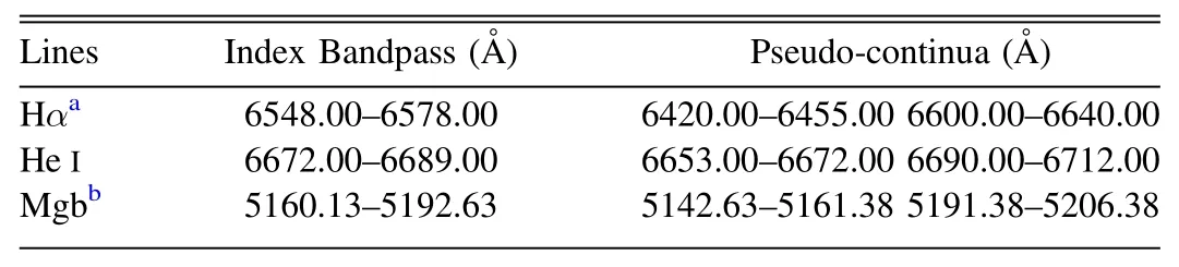
Table 1The De finition of Equivalent Width

3.Identi fication of OBA Stars

3.1.The Initial Sample

We collected a sample of over 800,000 stars from LAMOST-MRS.In these objects,～500,000 have st ellar par amet er s8http://dr7.lamost.org/v1.3/cataloguederived from the LAMOST stellar parameter pipeline(LASP)(Luo et al.2015,A.L.Luo et al.2021,in preparation).LASP adopts computational algorithms of the Correlation Function Initial(Du et al.2012)and the Universite de Lyon Spectroscopic analysis Software(Koleva et al.2009),and obtainsTeffby minimizing theχ2between model spectra and observed spectra(Luo et al.2015).Due to the limitation of the pipeline,only stellar parameters for A and later type stars,i.e.,withTeffin range of 3100–8500 K,are given(Wu et al.2011).The typical uncertainty ofTefffor LRS from the LASP is 110 K(Wu et al.2014;Gao et al.2015),while that for MRS was not given yet.Zhang et al.(2020a)showed that the accuracy of simulated MRS spectra is similar to that of LRS for stars with solar abundances.

Since we were only concerned with the multiplicity of earlytype stars in this paper,we then eliminated stars with spectral type later than A5,i.e,with estimatedTeff＜8000 K given by the LASP.We included～300,000 stars without estimatedTeffin our initial sample because many early-type stars are in this part.However,a broad range of stars of various spectral types is mixed in such a sample.We thus eliminated spurious latetype stars in our sample by the following selection criteria.

3.2.Removing Stars Later Than A5

The classic method to classify stars with MK types is comparing their spectra manually with standard stars(Gray&Corbally 2009,2014).This approach is hard to handle with huge samples of observations.The photometric color indices are also widely used in classifying stars,but such a method is heavily affected by interstellar reddening.It is dif ficult to calibrate the reddening in the deep sky(Liu et al.2015).In this work,we thus employed the EWs of several lines to exclude late-type stars(later than A5)in our sample(Liu et al.2015).The EW for a given spectral line is de fined as whereFline(λ)is the flux of the spectral line at a given wavelengthλ,andFcon(λ)is the flux of pseudo-continuum and is derived from linear interpolation of fluxes on both sides of a selected line bandpass(Worthey 1994).Due to high effective temperatures for early-type stars,not many line features are shown in the LAMOST-MRS spectra.Consequently,we measured the EW of the Hαλ6564?,He Iλ6679?and Mgb series(Liu et al.2015,2017).Table 1 features the information on index bandpass and the two continua bands for these lines(Cohen et al.1998;Liu et al.2015).Figure 1 displays the distributions for our initial sample as the black points in(EWMgb,EWHα)and(EWHeI,EWHα)panels.

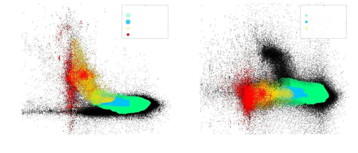
Figure 1.The black dots are our initial sample.The blue and green dots represent late A-and F-type stars in the 1σand 2σcontour region of Figure 2,respectively.The yellow dots signify the G-type stars,and the red dots correspond to M-and K-type stars(for details,see Section 3.2).

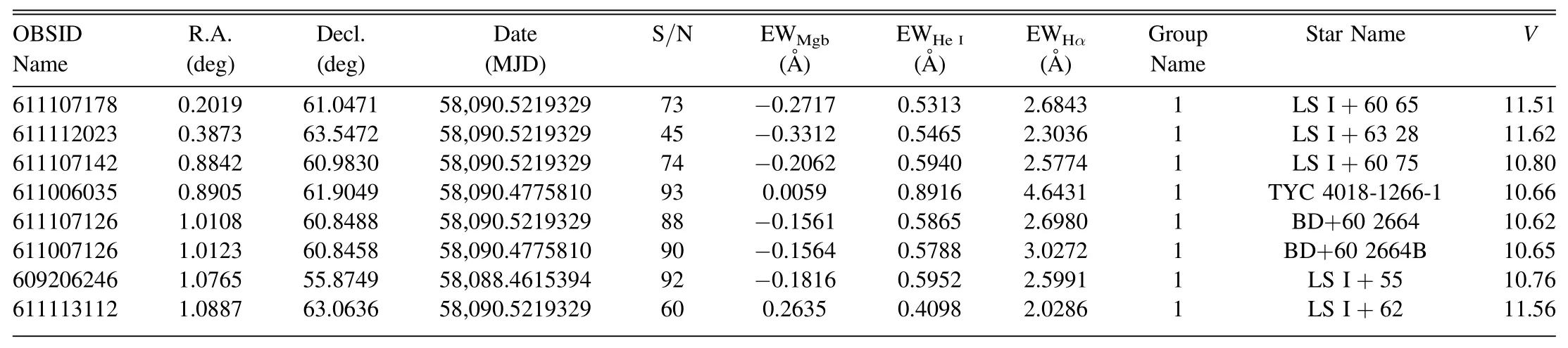
Table 2The OBA Catalogs

Table 3Numbers of OBA Stars and the Time-domain Observation Stars

As the first step,we removed late A-and F-type(LAF)stars from the sample.To do this,we chose LAF stars in LAMOSTMRS,i.e.,with 6500 K≤Teff≤8000 K(Habets&Heintze 1981)and calculated the EWs of Hα,He I and Mgb for these stars.Figure 2 depicts the probability density distributions of the EWs in the(EWMgb,EWHα)plane(left panel)and in(EWHeI,EWHα)plane(right panel),respectively.The color bar on the right side indicates the probability density.The distribution of the LAF stars within the 1σ(68.27%,black),2σ(95.45%,green)and 3σ(99.73%,blue)regions are shown with black,green and blue lines respectively.

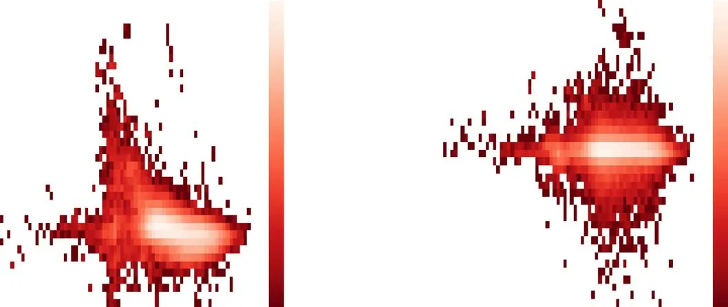
Figure 2.The distribution of late A-and F-type stars in Hαvs.Mgb panel(left)and Hαvs.He I panel(right)in which the color-bar represents the probability density of the distribution.The black and green(blue)contour lines signify the contours of stars in 1σand 2σ(3σ)respectively.

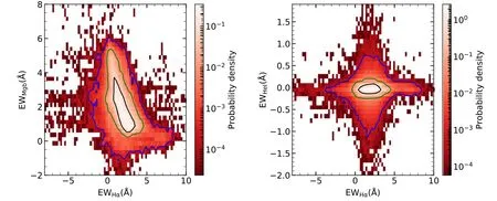
Figure 3.The distribution of G-type stars in the Hαvs.Mgb panel(left)and Hαvs.He I panel(right)in which color-bar represents the probability density of the distribution.The black and green(blue)contour lines signify the contours of stars in 1σand 2σ(3σ).

In principle,we can remove most LAF stars from the sample if we discard the objects located in the region enclosed by the 2σline.However,if we do like this,we will lose a majority of early A-type stars in our sample,since the spectral features of F-type stars are similar to those of A-type stars,resulting in EW density distributions of F-type stars being indistinguishable from those of A-type stars.This can be clearly seen in Figure 1 where we overlapped LAF stars within the region of 1σand 2σ.So,we only eliminated LAF stars within the region enclosed by the 1σline in this step.9The region enclosed by the 1σline corresponds to 6978 stars shown as blue dots of Figure 1,while 2σencloses 135,732 stars as marked by green dots in Figure 1.We will double-check our final sample by visually examining the individual spectrum to exclude any spurious late-type star spectrum after applying all the criteria.

We applied a similar approach to exclude G-type stars withTeffin the range of 5200–6500 K(Habets&Heintze 1981).The probability density distributions for the G-type stars are depicted in Figure 3.Stars within 2σ,corresponding to the 95.45%con fidence level regions of the distribution,were excluded from the sample.

Because the LAMOST-MRS pipeline does not assignTeffto stars cooler than 3100 K,we are not able to apply the above method to remove M-and K-type stars.We cross-matched the stars in our sample using their coordinate designation with the Two Micron All-Sky Survey(2MASS)database(Cutri et al.2003)(within 3″),and obtained the reddening-free quantityQ(Q=(J-H)-1.70(H-KS))for the common stars.Negueruela&Schurch(2007)suggest that for M-and K-type stars,theQvalues are expected to be within a range of 0.4 to 0.5.Figure 4.Left panel:Distribution of the OBA type stars referenced by previous literatures in He I(6679?)vs.Hα(6565?)panel.The black triangles and circles indicate the O-and A-type stars,respectively.The colored star symbols stand for the different sub-types of B stars.The red lines mark the boundaries between groups.Right panel:The distribution of our final OBA candidates in the four groups of LAMOST-MRS data.The gray lines are the boundaries of the groups.Therefore,we selected stars satisfying this condition(displayed as red dots in Figure 1)to remove them from our sample.

Since the He I line pro file appears prominent in spectra of early-type stars,the line pro file gradually decreases in strength toward cooler stars and is mostly absent in the spectra of A-type stars.We thus selected the stars with measured EWHeI≤0.1 to remove any spurious late-type stars further.We use the information onTeffgiven by Gaia Data Release 2(DR2)10Andrae et al.(2018)apply an empirically-trained data-driven method to give the T eff of Gaia DR2.Due to the limit of training data,T err is in the range of 3000–10,000 K,and the typical accuracy is 324 K.to remove any missing late-type stars in the sample.We cross-matched the data set within 3″with Gaia DR2 to find common stars and then keep stars with estimatedTeff≥7300 K(F0)to be our final sample of early-type stars(Habets&Heintze 1981).11Although there are some arguments on the effective temperature given by Gaia,especially for OB stars,we only use them to remove late type stars,i.e.,with T eff≤7300 K.The real temperature is not considered here and has little effect on our results.

Lastly,through visual inspection of the individual spectrum in the sample,we found a residual contamination rate of latetype stars of about 1.6%in our sample.We then removed these stars,as well as spectra displaying emission pro files from the sample.In our final data set,we collected a sample of 9382 stars with signal-to-noise ratio(S/N)＞40.All the targets have a simple magnitude cut-offG～13(Liu et al.2020).

3.3.The Sample Grouping

In order to investigate the relationship of the multiplicity properties of early-type stars as a function ofTeff,we first need to group the OBA stars in our sample based upon theirTeff.However,no information on theTefffor these stars is available.Also,it is dif ficult to distinguish the spectra of late O-type stars from those of early B-type stars due to their color degeneracy(Maíz-Apellániz et al.2004)(or late B-type from early A-type stars,Liu et al.2015).Liu et al.(2019c)has demonstrated the applicability of using the spectral line indices to classify the spectral types of early-type stars in LAMOST-LRS.We thus adopted their approach to divide the stars in our sample into four catalogs inTeff.We collect a sample of template stars with known spectral types from literature(Hiltner 1956;Nesterov et al.1995;Negueruela&Marco 2003;Beerer et al.2010;Comerón&Pasquali 2012;Hou et al.2015;Liu et al.2019c).We cross-matched these stars with the LAMOST-MRS database to collect spectra of common stars,including 136 O-type stars,308 B-type stars and 898 A-type stars.We then measured their EWs of the Hαλ6564?and He Iλ6679?line pro files.In Figure 4,on the left panel,we plot the measured EWs in the(EWHeI,EWHα)plane,in which the triangles and circles indicate the EW measurements for O-and A-stars,respectively,and the star symbols represent the B-type stars.The vertical color bar on the right side signi fies the spectral sub-type distribution of B-type stars.Based upon the EWs,we group the stars into four groups of T1,T2,T3 and T4.As depicted in the right panel of Figure 4,the stars in group T1 comprise mostly O-B4-type stars,and most B5-type stars reside in group T2,while the majority of B7-type stars are distributed in the region T3.Cooler stars of B8-A4 are illustrated in region T4 on the plot(Guo et al.2021).On the right panel,we adopted the criteria to group our observed OBA stars in the sample.

Sota et al.(2014)presented a spectral classi fication for a catalog of 448 Galactic O-type stars from GOSSS.We cross-matched the LAMOST-MRS catalog with GOSSS,and only four non-emission stars were found.We also crossmatched the LAMOST catalog with the published 146 OB stars from Kiminki et al.(2007),and only 14 common sources were found.All the 18(4+14)sources above with the spectral type from O5.5 to B1 are in the T1 group indicating that it is reasonable to adopt the method to obtain the four groups.

In Table 2,we list the observation ID for each of the stars,their coordinates,Modi fied Julian Date(MJD),S/N,the associated EW measurements for all three line pro files,their classi fied group index,star name andVmagnitude(from SIMBAD).The number of stars within each group is listed in Table 3.

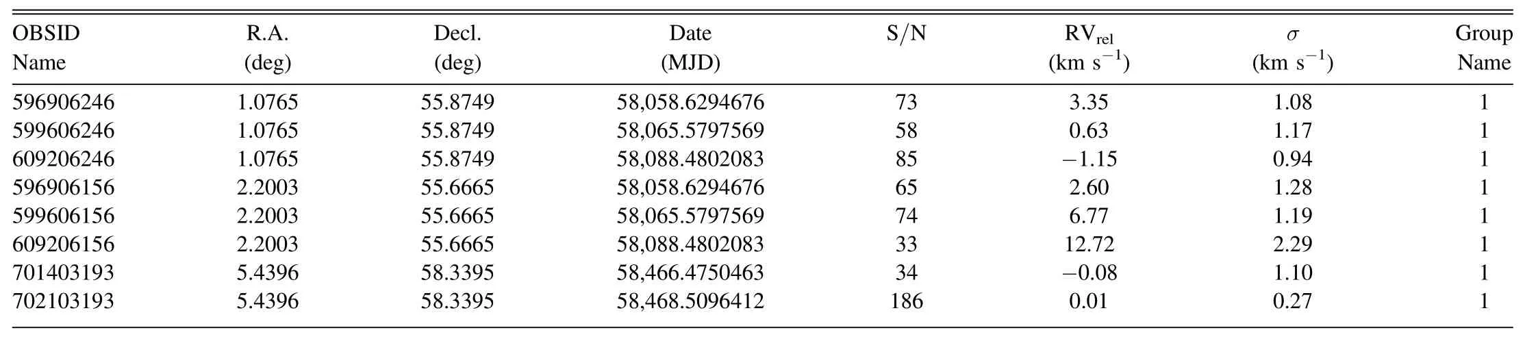
Table 4The RV Catalogs

4.Radial Velocity Measurements and Analysis

4.1.RV Measurements

The RV measurement is a vital ingredient of this study since detecting signi ficant RV variations relies on RV differences.We adopted the maximum likelihood method described in Xiong et al.(2021)to measure the relative RVs.We brie fly describe the procedures as follows.For each star,a set of multiple exposures was obtained from the LAMOST-MRS,and we selected the exposure with the highest S/N as the template spectrum.The likelihood distribution for theith star observed at timetof the relative radial velocity(RVrel)is

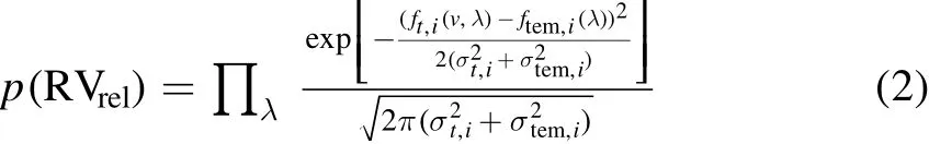
whereftem,i(λ)andft,i(v,λ)represent the observed flux of a template spectrum and individual exposure,respectively,while σtem,i(σt,i)is the observed flux error of a template spectrum(individual exposure).A Gaussian fit was applied to each of the likelihood distribution functions,and we estimated the peak value of the fit as our RVrelmeasurement,and the uncertainty(σunc,i)of the RV measurements was obtained from the standard deviation of the Gaussian fit.Such an approach yields a systemic error of 0.25 km s-1(σsys).

Systematic errors exist among the RVs obtained from spectra collected by different spectrographs and exposures of LAMOST-MRS surveys(Liu et al.2019b;Zhang et al.2021).Therefore,we matched our catalog,including 2911 early-type stars,with the one from Zhang et al.(2021)and found that the median values of the RVs before correction and after correction are～0.6 km s-1.In the paper,we used a strict criterion to select the binary stars(see Equation(3)).This means that the in fluence of uncorrected RV on the derived binary fraction is little and can be ignored.We also compared the observed binary fraction based on the RVs from Zhang et al.(2021)and Xiong et al.(2021)and found that the difference between the observed binary fractions derived in the two ways is less than 1.5%.Therefore,we kept using the RVrelfrom Xiong et al.(2021)in the following analysis.

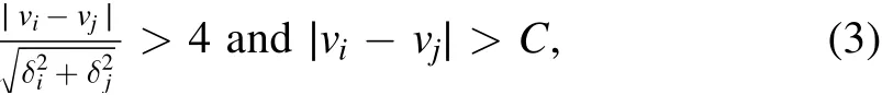
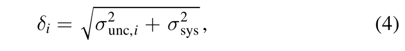
In our final sample of 9382 candidates,only 2911 stars were observed more than twice(see column 3 in Table 3).The following analysis of this work is based on the sample of 2911 stars.The measured RVreland the uncertainties(σunc,i)for each star are tabulated in Table 4.The number distribution of the stars as a function of observing baseline is depicted in Figure 5.In Figure 6,we display the number of observations for stars in each temperature group.

4.2.Criterion for Binarity

We adopted the method from Sana et al.(2013)(see their Equation(4))to identify binary candidate systems in our sample(Sana et al.2012;Dunstall et al.2015;Banyard et al.2021;Mahy et al.2021).We considered a star as a binary if RVrelsatis fies the criterion

wherevi(j)andδi(j)are the RVreland the associated uncertainty measured for the spectrum at epochi(j)respectively.Here we divided the uncertainty into two parts

whereσunc,iis the uncertainty of theith star observed at timetwhileσsysis the typical systematic error(see Section 4.1).

The thresholdCis adopted to eliminate the stars with signi ficant RV variation caused by pulsation of the photosphere or atmospheric activity.Sana et al.(2013)and Dunstall et al.(2015)report that this value is assigned from a kink on the RV distribution plot(see Figure 6 in Sana et al.2013).We followed a similar approach of searching for a possible kink from the RV distribution to constrain the thresholdCvalue.However,no such pattern is apparent in our RV plot shown in Figure 7.In order to eliminate the pulsational variable stars in our sample,we adopted the typical period and RV amplitude ofδScuti type stars12Here we care about pulsating variable stars with OBA types,that is,β Cephei,Slowly Pulsating B(SPB)andδScuti.We cross-matched the catalog of Kochanek et al.(2017),GAIA Collaboration et al.(2019)and Chen et al.(2020)with our catalog,but only found five sources in common(we have eliminated them).The contamination byδScuti stars in our sample is much more likely than that byβCephei and SPB(Watson et al.2006;Chen et al.2020),so we adopted the threshold value derived fromδScuti in this paper.This value is larger than that forβCephei(Stankov&Handler 2005)and likely leads to a lower observed binary fraction.However,we aim to remove contamination of pulsating variable stars as much as possible to ensure the purity of the sample.It has little effect on the intrinsic binary fraction after the MCMC correction.to perform a Monte-Carlo simulation to constrain the thresholdCvalue,resulting in a value of 15.57 km s-1(Breger 1979,2000;Fernie 1994).

4.3.Observed Binary Fraction

According to the criterion(3),the observed binary fractionsof these four groups are 24.6%±0.5%,20.8%±0.6%,13.7%±0.3%and 7.6%±0.3%,respectively.Thefor the stars in each group is plotted as red dots and displayed in Figure 8.The error bars were estimated through bootstrapanalysis from Raghavan et al.(2010).The result af firms thatdecreases as the spectral type moves from O-type to A-type stars.

Figure 5.The number distribution of stars as a function of observational baseline.Panels(a)–(d)represent the stars in groups T1,T2,T3 and T4,respectively.

Figure 6.Number distribution for observations with S/N＞40.Panels(a)–(d)represent the stars in groups T1,T2,T3 and T4,respectively.It indicates that 59%of stars have two observations,and 10%have five or more observations.

Figure 7.The varied fraction of systems below and above the critical C.The solid line indicates the varied fraction of systems with different thresholds of C.The dash-dotted lines signify the low-amplitude RV variable fractions of systems with different thresholds of C.The vertical red dashed lines represent the final adopted threshold of C=15.57 km s-1.

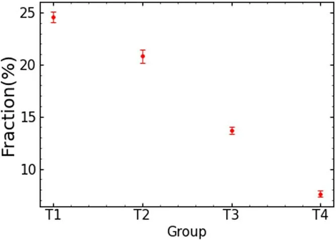
Figure 8.The observed binary fractions for the four groups.

In fact,this way may underestimate the fraction of binary stars,since the binaries with relatively small RV variations in the measurements based on the LAMOST-MRS spectra are missed.In addition,if the phase differences of the spectroscopic observations of LAMOST are small,even the binary stars with large RV amplitudes might be missed.Besides,a different thresholdC-value may affect the result ofbut all the bias above can be corrected when we investigate the intrinsic binary fraction through Monte-Carlo simulations in the next section.

5.Intrinsic Multiplicity Properties

As stated above,the observedbdepends on the thresholdC-value.Moreover,based upon the observational baseline and cadence nature for stars in our sample,we may miss the detection of long period binary systems.In this section,we perform a series of Monte-Carlo simulations to correct such biases.

5.1.Monte-Carlo Method

Following the approach as noted by Sana et al.(2013),we need to adopt the Monte-Carlo simulation to construct synthetic cumulative distribution function(CDF)of RV variance(ΔRV is the maximum RV variance among individual exposure)andΔMJD(minimum timescale between the exposures).We assume the probability density distribution of orbital period(P)and mass ratio(q)of binary system satis fies the power-lawf(P)∝Pπandf(q)∝qκ, respectively.We modi fied the distribution of orbital period in a log-scale of(logP)∝(logP)πto linear form to be more sensitive to short-period binaries.In Table 5,we list the variable ranges for the parameters,and we set the step size to be 0.1 forπandκ,and 0.04 forfb.We adopt the initial mass function(Salpeter 1955)to describe the mass distribution of stars in our grouped catalogs of T1～T4.

Table 5The Range of Parameters used in the Monte-Carlo Simulation

Generally,six parameters are used to describe two-body kinetic systems in a Keplerian orbit:inclination(i),the argument of periastron(ω),true anomaly(ν),eccentricity(e),semimajor axis(a)and the epoch of periastron(τ).The inclination satis fies a probability distribution of sin(i)and is randomly drawn over an interval from 0 toπ/2.The argument of periapsis satis fies a uniform distribution and is randomly drawn from 0 to 2π.We useeηto describe the distribution and setηas-0.5,the same as in Sana et al.(2013).The semimajor axis depends on the orbital period(P).Theτis selected at random with the unit of days.

We followed the same method as discussed in Appendix C of Sana et al.(2013),and used our selected parameters with assigned range to perform the simulation to obtain cumulative distributions ofΔRV andΔMJD.We followed a similar approach as Sana et al.(2013)to obtain the global merit function (GMF) using the simulated CDFs and our observations.The final results are given by the projection of the GMFs,i.e.,π,κandfb.

5.2.Validation

In order to verify the robustness of applying the methodology from Sana et al.(2013)to our data set,we performed a self-consistency validation test,as well as testing for the suitability of adopting the GMF.

5.2.1.Self-consistency Test

To verify the self-consistency of our code,we collected the reported RV measurement of 360 stars from Sana et al.(2013)and obtained the optimalπ,κandfbvalues.The optimal values of the distribution were found to be π=-0.4±0.4,κ=-0.9±0.4 andfb=52±5%,shown in Figure 9,while Sana et al.(2013)reported their findings ofπ=-0.45±0.3,κ=-1±0.4 andfb=51%±4%.Considering the uncertainties of the parameters,our calculated values are in agreement with those of Sana et al.(2013).

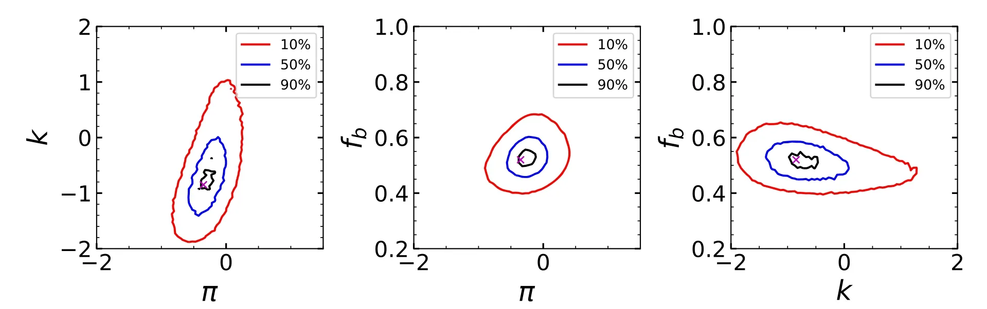
Figure 9.Projections of global merit function de fined byπ,κand fb from the data of Sana et al.(2013).The pink x indicates the absolute maximum.The loci of 10%,50%and 90%con fidence levels of global merit function are displayed in the red,blue and black contours,respectively.

5.2.2.The Applicability of the GMF

In order to test the applicability of applying the GMF to determine the probability density distribution of sample stars from the LAMOST-MRS,we first constructed 68 synthetic CDFs ofΔRV andΔMJD using the input sets ofπ,κandfb.The choices of such values are listed in Table 6.Based upon the constructed input synthetic CDFs and results discussed in Section 5.1,we then obtained the 68 projections of GMFs.A comparison of the output synthetic GMFs to the input parameters ofπ,κandfbis displayed in Figure 10.

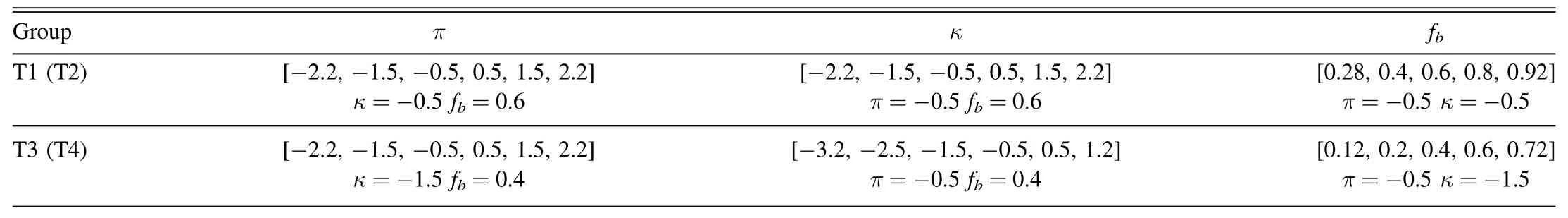
Table 6The Input Parameters ofπ,κand fb

The top two rows show the constrained results for the groups in T1 and T2 from the synthetic CDFs distribution,while the bottom two rows are for the groups in T3 and T4.We found that the results of stars in groups T3 and T4(12 and 14 points)are better constrained than those from T1 and T2(7 and 6 points),in which the point represents the constrained result.The results indicate that the method is applicable for sample stars in groups T3 and T4,but not for stars in groups T1 and T2,especially forκ.In order to explore the reasons for the unconstrainedκvalue,we repeat the analysis above using theobservedCDFs ofΔRV andΔMJD for stars in group T1.The results are displayed in the top panel of Figure 11.We note that theκvalue is still not well constrained.We thus further explore the possibleκvalues by extending the range to-4.5～0.5.The results are displayed in the bottom panel of Figure 11,where we see thatκis still unconstrained.The results for T2 are similar to those of T1.This indicates that the initially selected range ofκvalues is independent of whether it can be constrained or not.This might be explained by the small value of sample size(N)for groups T1 and T2,which is an initial input of the binomial distribution of the GMF.

Considering that a large number of unconstrainedκvalues for stars in the groups T1 and T2 may affect the results of other parameters,we fixed theκvalue to guarantee the reliability of other parameters(Sana et al.2013).According to the initial mass function,the population of late-type stars shows an increasing trend toward small stellar mass.Therefore,the sample size of early-B type stars is larger than that of the O-type stars for the stars in groups T1 and T2.We thus adopt the value ofκfrom Dunstall et al.(2015),i.e.,κ=-2.8 for early B-type stars and repeat the analysis above again to verify the applicability of the method.Based upon the validation tests,we then obtained the final results ofπandfbfrom the GMFs by repeating the procedures as mentioned in Section 5.1,except that we now fixed the value ofκto be-2.8 for sample stars in groups T1 and T2.

5.3.Results and Discussion

5.3.1.Results

The GMF projections ofπ,κandfbfor stars in groups T1 to T4 are depicted in Figure 12.The red,blue and black contours indicate the loci of 10%,50%and 95%con fidence levels of GMF.The intrinsic binary fractions of these four groups are 68%±8%,52%±3%,44%±6%and 44%±6%,respectively.Theπvalues of these groups are-1±0.1,-1.1±0.05,-1.1±0.1 and-0.6±0.05,respectively.Theκvalues of T3 and T4 are-2.4±0.3 and-1.6±0.3,respectively.

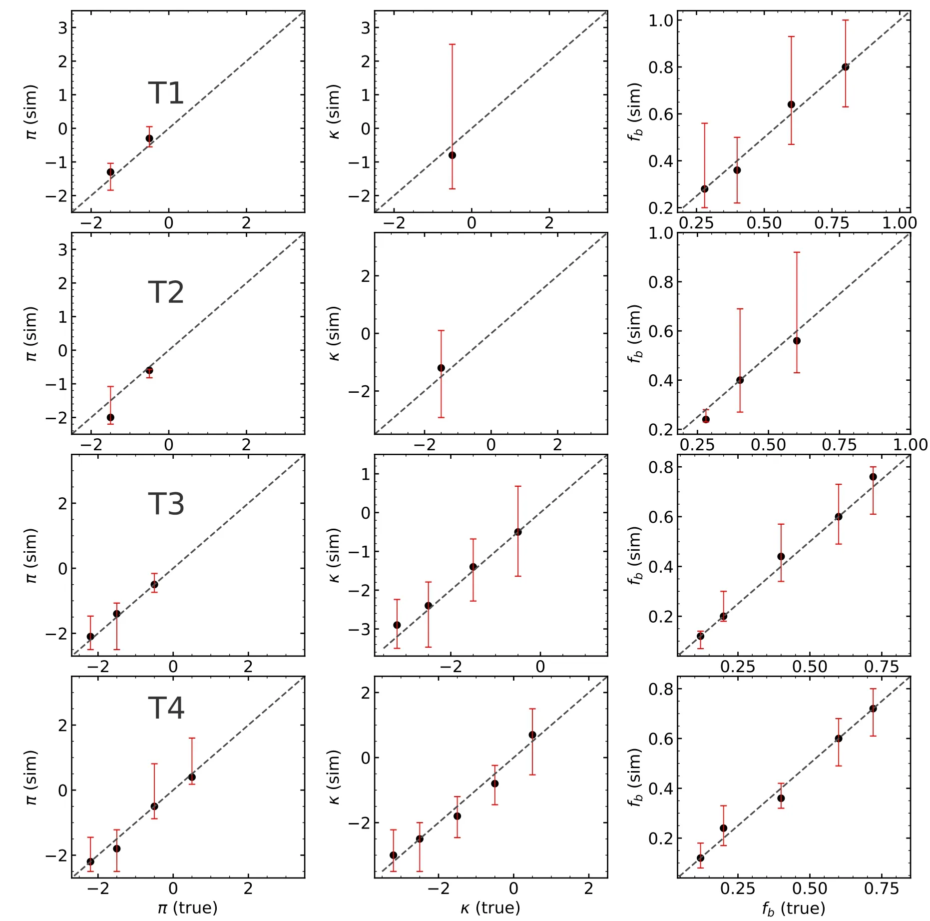
Figure 10.Comparison for testing the suitability of the global merit function.The x-axis represents the input value from Table 6 while the y-axis corresponds to the output constrained values after using the Monte-Carlo simulation,in which we did not include the points with unconstrained results.The errors are given by the upper and lower boundaries of 50%con fidence levels.

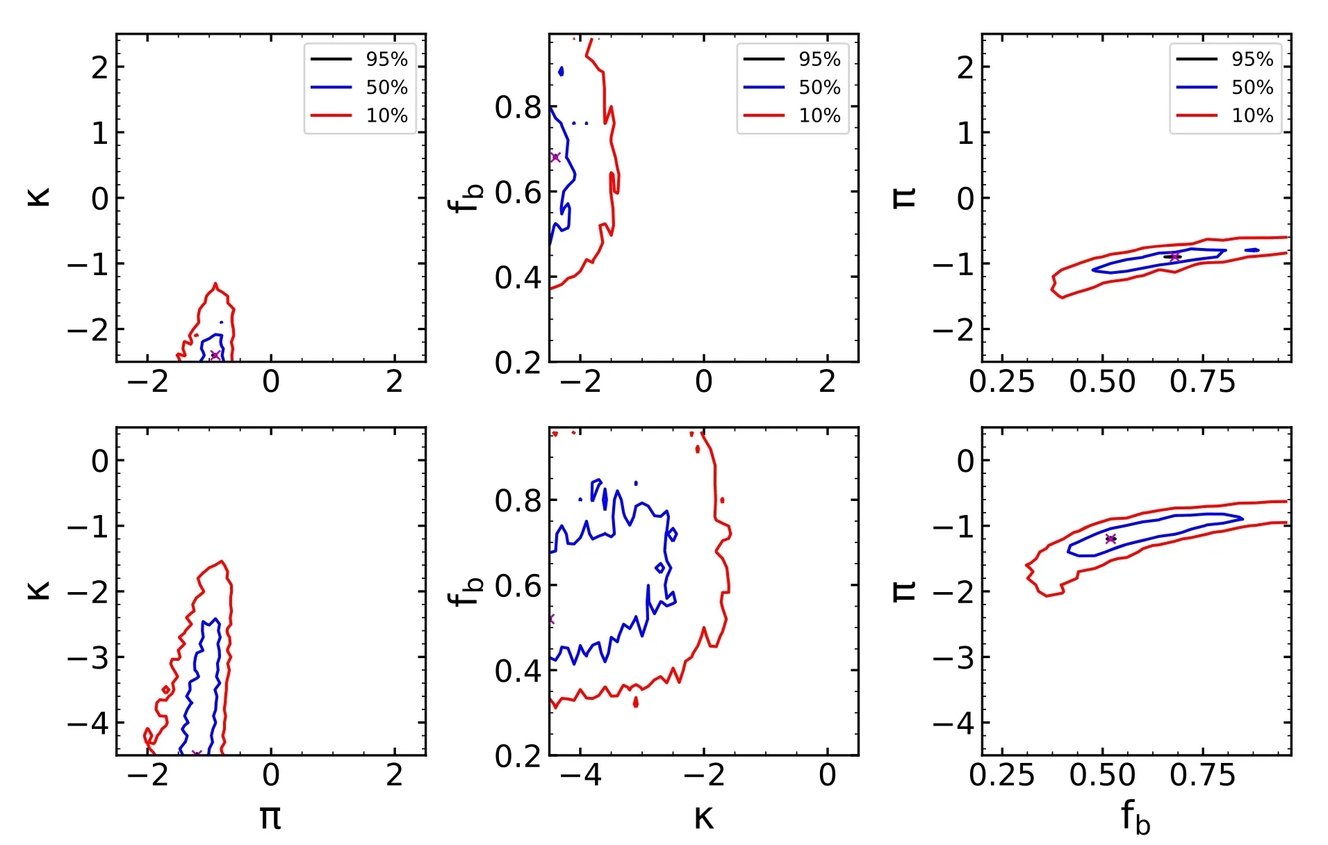
Figure 11.The projections of global merit function for stars in groups T1,but with different ranges ofκ.Theκrange of[-2.5,2.5]is in the upper panel while[4.5,0.5]in the bottom panel.

Note that,although the thresholdC-value does affect the observed binary fractionfbo,the bias has been corrected here for the intrinsic fraction since the sameC-value is used in our Monte-Carlo simulations.Mahy et al.(2021)analyzed different thresholdC-values using the Monte-Carlo method from Sana et al.(2013)to see whether different choices ofC-value affect the final estimation for the intrinsic binary fraction or not.They found that the adopted thresholdCdoes not affect the final results unless signi ficant contamination exists by false-positive RV measurements.

5.3.2.Discussion

Our intrinsic binary fractions(red squares)for stars in groups T1 to T4 are shown in Figure 13,and the star mark is the result of Galactic O-type stars from Sana et al.(2012).The final result indicates that the intrinsic binary fractions decrease toward latetype stars.

We are also interested in investigating the distribution of orbital period as a consequence of spectral type(onTeff).We then plot the orbital period distribution in the left panel of Figure 14 for sample stars in groups T1 to T4(shown as solid black line,green dashed line,black dashed line and black dotted line,respectively)as well as similar over-plotted distribution by adopting the results repeated from Sana et al.(2013)in blue and Dunstall et al.(2015)in red.We plotted each work’s orbital period distribution with the upper and lower uncertainty ranges by adding and subtracting the uncertainty from the best-estimated values,respectively,in the right panel of Figure 14.It seems that the distribution of group T4 is more flat.

Ourκ(red squares)distributions are shown in Figure 15.The star mark is the result of Sana et al.(2013),and the triangle represents the result of Dunstall et al.(2015).All of them have large error bars,and no signi ficant correlation is found.

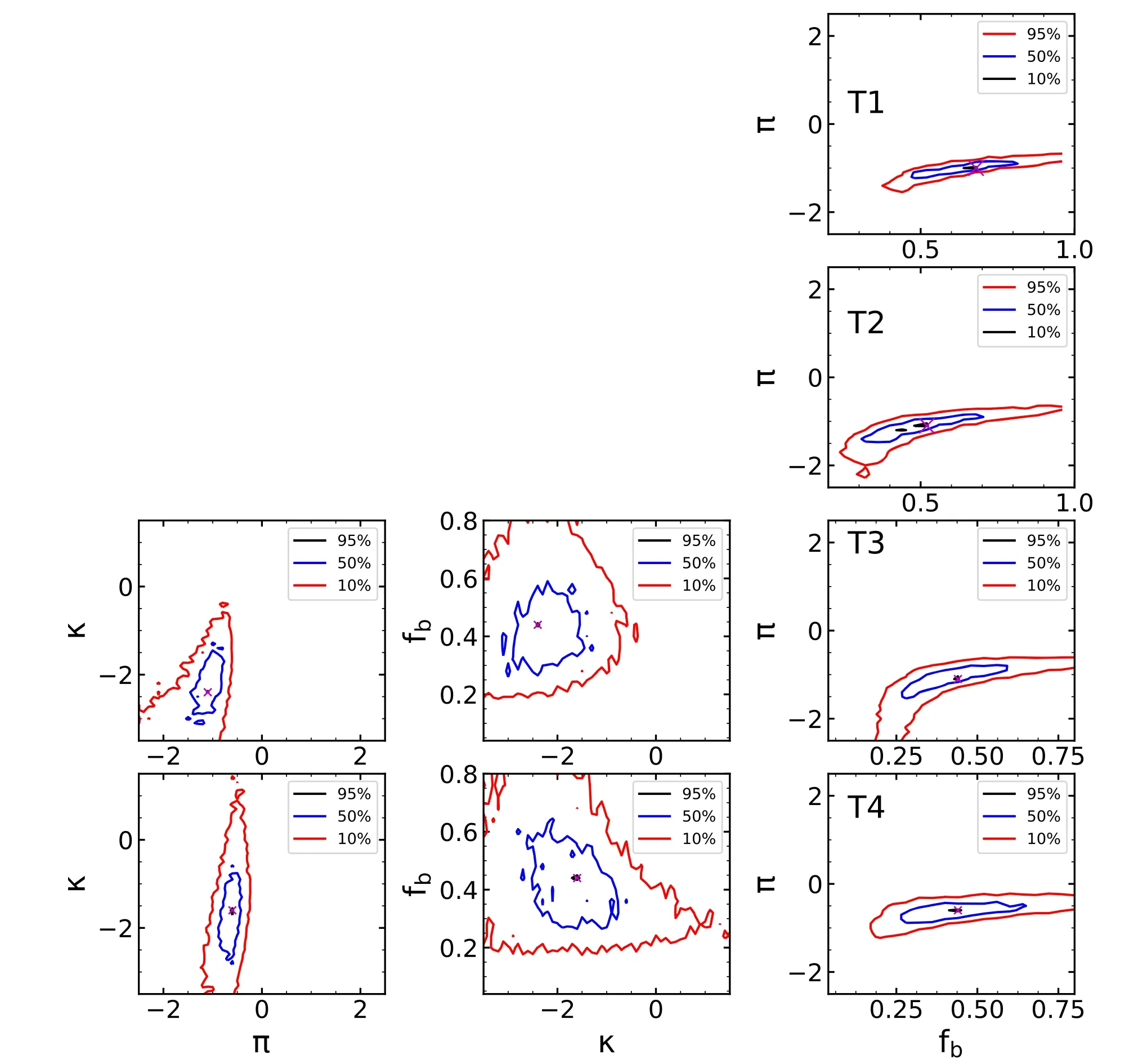
Figure 12.The projections of GMFs for stars in groups T1 to T4.The left and middle(right)panels are the projections ofπandκ(fb)for stars in groups T1 to T4.

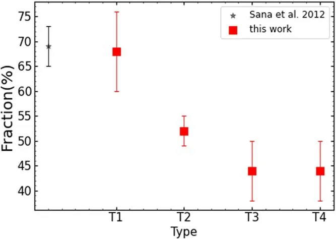
Figure 13.Comparison of our intrinsic binary fractions with previous works.The red squares represent the intrinsic binary fractions in our work for stars in groups T1 to T4,and the star mark is the result of Galactic O-type stars from Sana et al.(2012).

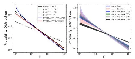
Figure 14.Comparisons of orbital period distribution with the results from previous works.In the left panel,the blue line represents the result of Sana et al.(2013),and the red one corresponds to that of Dunstall et al.(2015).The black and green lines stand for the result of this work.The right panel displays the upper and lower uncertainty orbital period distribution for each work.

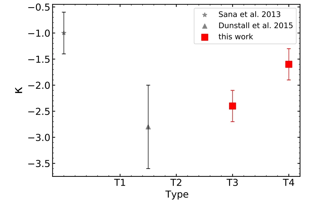
Figure 15.Comparison ofκin T3 and T4 with previous works.The star mark and the triangle represent the result of Sana et al.(2013)and Dunstall et al.(2015),respectively.

6.Conclusions

We identi fied 9382 early-type stars from the LAMOST-MRS data set based on the EWs.These early-type stars were roughly classi fied into four groups of T1,T2,T3 and T4 based upon theirTeffin descending order.The number of stars in each group is 1138,1092,2649 and 4503,respectively.Then we calculated the RVrelof multi-epoch early-type stars by using the Maximum Likelihood Estimation method and then identi fied spectroscopic binaries with signi ficantΔRV.The observed binary fractions of these four classi fications are 24.6%±0.5%,20.8%±0.6%,13.7%±0.3%and 7.4%±0.3%,respectively.

We utilized a Monte-Carlo method to correct observational bias and constrain the intrinsic properties,including the binary fraction,distributions of orbital period and mass ratio.The intrinsic binary fractions of stars residing in T1 to T4 are 68%±8%,52%±3%,44%±6%and 44%±6%,respectively.The orbital period distributions follow the power-law off(P)∝Pπ,and theπvalues for each group are-1±0.1,-1.1±0.05,-1.1±0.1 and-0.6±0.05,respectively.The mass ratio distributions follow the power-low off(q)∝qκ,and theκis unconstrained for groups T1 and T2 while for T3 and T4 we reported theκhas values of-2.4±0.3 and-1.6±0.3,respectively.

Based on the binary fraction results,the early-type massive stars are likely to have a higher chance of hosting companion stars compared to late-type,low-mass stars.The multiplicity properties as a basic physical input of BPS not only have an impact on the final results of BPS but also allow us to better understand the evolution of massive stars.

For future work,we expect to better constrain these multiplicity parameters as more observations will be made possible.

Acknowledgments

This work is supported by the Natural Science Foundation of China(NSFC,Grant Nos.11733008,12090040,12090043,11521303,12125303),Yunnan Province and the National Tenthousand Talents Program.C.L.acknowledges National Key R&D Program of China No.2019YFA0405500 and the NSFC with Grant No.11835057.

The authors gratefully acknowledge the“PHOENIX Supercomputing Platform”jointly operated by the Binary Population Synthesis Group and the Stellar Astrophysics Group at Yunnan Observatories,Chinese Academy of Sciences.

The Guoshoujing Telescope(the Large Sky Area Multi-Object Fiber Spectroscopic Telescope,LAMOST)is a National Major Scienti fic Project built by the Chinese Academy of Sciences.Funding for the project has been provided by the National Development and Reform Commission.LAMOST is operated and managed by the National Astronomical Observatories,Chinese Academy of Sciences.

This work is also supported by the Key Research Program of Frontier Sciences,CAS,Grant No.QYZDY-SSW-SLH007 and the science research grants from the China Manned Space Project with No.CMS-CSST-2021-A10.

ORCID iDs

Yanjun Guo, https://orcid.org/0000-0001-9989-9834

Jianping Xiong https://orcid.org/0000-0003-4829-6245

Luqian Wang https://orcid.org/0000-0003-4511-6800