Xiaoyue Cao ,Ran Li,J.W.Nightingale,Richard Massey,Andrew Robertson,Carlos S.Frenk,Aristeidis Amvrosiadis,Nicola C.Amorisco,Qiuhan He,Amy Etherington,Shaun Cole,and Kai Zhu

1 National Astronomical Observatories,Chinese Academy of Sciences,20A Datun Road,Chaoyang District,Beijing 100012,China;ranl@bao.ac.cn

2 School of Astronomy and Space Science,University of Chinese Academy of Sciences,Beijing 100049,China

3 Institute for Computational Cosmology,Physics Department,Durham University,South Road,Durham,DH1 3LE,United Kingdom

Received 2021 September 17;revised 2021 October 22;accepted 2021 October 27;published 2022 February 2

Abstract The elliptical power-law model of the mass in a galaxy is widely used in strong gravitational lensing analyses.However,the distribution of mass in real galaxies is more complex.We quantify the biases due to this model mismatch by simulating and then analyzing mock Hubble Space Telescope imaging of lenses with mass distributions inferred from SDSS-MaNGA stellar dynamics data.We find accurate recovery of source galaxy morphology,except for a slight tendency to infer sources to be more compact than their true size.The Einstein radius of the lens is also robustly recovered with 0.1%accuracy,as is the global density slope,with 2.5%relative systematic error,compared to the 3.4%intrinsic dispersion.However,asymmetry in real lenses also leads to a spurious fitted“external shear”with typical strengthγext=0.015.Furthermore,time delays inferred from lens modeling without measurements of stellar dynamics are typically underestimated by～5%.Using such measurements from a sub-sample of 37 lenses would bias measurements of the Hubble constant H0 by～9%.Although this work is based on a particular set of MaNGA galaxies,and the speci fic value of the detected biases may change for another set of strong lenses,our results strongly suggest the next generation cosmography needs to use more complex lens mass models.

Key words:galaxies:structure–galaxies:halos–gravitational lensing:strong

1.Introduction

Strong gravitational lensing is a phenomenon whereby the light of a background source galaxy is highly distorted by the gravitational field of a foreground lens galaxy,such that the source is observed as multiple images or in extended arc structures.Over the last few decades,strong gravitational lensing has become a powerful tool for astronomers,for example it has been used as a“cosmic telescope”to observe magni fied high-redshift sources(Newton et al.2011;Shu et al.2016b;Cornachione et al.2018;Blecher et al.2019;Ritondale et al.2019a;Cheng et al.2020;Marques-Chaves et al.2020;Rizzo et al.2020;Yang et al.2021),as a probe of the mass structure and substructure of foreground lenses(Treu et al.2006;Koopmans et al.2006;Gavazzi et al.2007;Bolton et al.2008b;Vegetti&Koopmans 2009;Auger et al.2010;Bolton et al.2012;He et al.2018;Nightingale et al.2019;He et al.2020b;Du et al.2020),as a tool to constrain the nature of dark matter(Mao&Schneider 1998;Vegetti et al.2012,2014;Li et al.2016,2017;Ritondale et al.2019b;Gilman et al.2019,2020;He et al.2020a;Enzi et al.2020)or as an independent method for cosmological parameters inference(Suyu et al.2013;Chen et al.2019;Birrer et al.2020;Millon et al.2020;Wong et al.2020).

Currently,thousands of strong lensing candidates have been discovered in large sky surveys(Bolton et al.2006a;Cabanac et al.2007;Brownstein et al.2012;Gavazzi et al.2012;Shu et al.2016a,2017;Para ficz et al.2016;Petrillo et al.2017;Cao et al.2020;Huang et al.2020;He et al.2020c;Li et al.2020).When high-resolution imaging is also available,it is possible to pin down the lens potential at the location of the multiple images to within a few percent(Chen et al.2016;Suyu et al.2017);infer the Hubble constant with～7%precision(Suyu et al.2010,2013);detect dark matter subhaloes of masses～108–109M⊙(Vegetti et al.2010,2012);and resolve～100 pc morphological structures in high redshift(z?2)source galaxies(Shu et al.2016b;Ritondale et al.2019a).

A key step toward all these scienti fic goals is to infer an accurate model of the lens mass distribution.This is challenging for a number of reasons,for example,the“source-position transformation”(SPT),whereby different lens mass models can produce almost the same lensed observations by simultaneously adjusting the distribution of lens mass and source light(Schneider&Sluse 2014).A well-known case of the SPT is the“mass-sheet transformation”(MST,Falco et al.1985),in which a rescaling of the lens’surface mass density by a factorλ,the simultaneous addition of a constant mass sheet with convergence(1-λ)and a rescaling of the angular size of the source by a factor ofλ,leaves the resulting lensed image unchanged except for a time delay.Schneider&Sluse(2013)show an example of the SPT transformation,where an elliptical power-law(EPL)mass model is fitted to a mock lens composed of a Hernquist stellar mass pro file(Hernquist 1990)and a generalized NFW(gNFW,Navarro et al.1996;Zhao 1996;Wyithe et al.2001;Cappellari et al.2013)dark matter mass pro file.Although the power-law mass model provides a good fit to the position of the lensed images and the central velocity dispersion of the lens galaxy,the inferred density pro file and time delays are signi ficantly offset from the truth due to the mismatch between the EPL and the more complex input lens mass distribution.

Many studies use the EPL mass model to describe the density pro files of lens galaxies when modeling galaxy-galaxy strong lenses.In reality,the structure of the lens galaxies is more complex and may not exactly follow the power-law radial pro file or conform to assumptions like perfect elliptical symmetry.This simpli fied mass model will therefore introduce systematic errors into the lens modeling.Although Suyu et al.(2009)found that for the mass pro file of lens system b1608+656,the deviation from the EPL model is less than～2%.Schneider&Sluse(2013)argue that even if the true mass pro file deviates only slightly from a power law,it may have an impact on the inferred time delay of over～10%.

To investigate biases that could be introduced when using a simple parametric model to describe the mass distribution of(presumably complicated)observed lenses,one approach is to generate mock lenses using galaxies from cosmological hydrodynamic simulations and then measuring the systematic error caused by fitting a parametric model(such as the EPL model),by comparing the results with the ground truth values(Mukherjee et al.2018;Enzi et al.2020;Ding et al.2021).A limitation of this method is that cosmological simulations may lack suf ficient resolution to resolve the internal structure of the lens galaxy,with the softening length of these simulations being usually between 0.3 and 1 kpc(Genel et al.2014;Vogelsberger et al.2014;Crain et al.2015;Schaye et al.2015;Nelson et al.2015;Marinacci et al.2018;Naiman et al.2018;Nelson et al.2018;Pillepich et al.2018;Springel et al.2018).Works that simulate lenses in this way have noted density cores at the center of the simulated lenses that are not consistent with observed strong lenses(Rusin&Ma 2001;Keeton 2003;Winn et al.2004;Boyce et al.2006;Zhang et al.2007;Quinn et al.2016).

Moreover,recent observations of stellar kinematics show that the hydrodynamic simulations may underestimate the average density slope within the half-light radius of Early Type Galaxies(ETGs).Li et al.(2019)analyzed the average inner density slope of more than 2000 galaxies in the SDSS-IV MaNGA survey,using the mass reconstructions given by the Jeans Anisotropic Multi Gaussian Expansion(JAM)dynamics modeling from Li et al.(2018a).They demonstrated that hydrodynamic simulations underestimate the average slope by about 10%–20%for massive ETGs.

In this work,instead of relying on ETGs from cosmological hydrodynamic simulations to make mock lens samples,we select 50 ETGs that are similar to The Sloan Lens ACS Survey(SLACS,Bolton et al.2006b)lenses in terms of mass and morphology from the integral field unit(IFU)observations of the MaNGA project and generate mock lenses based on the dynamical mass maps derived by the JAM method.We anticipate that these mock lenses contain many of the complexities found in the mass distributions of real galaxies(e.g.,non-symmetric mass structures)which the much simpler EPL mass pro file,often assumed for lens modeling,does not.Thus,this simulated data set will allow us to assess systematic errors in lens modeling due to assuming an unrealistic mass model.In particular,we evaluate the morphology of the source galaxy,the mass model parameters(Einstein radius,shear,inner density slope)of the lens galaxy,and the time delay measurement that is vital for studies of cosmography.

This paper is organized in the following way.In Section 2,we introduce the basic theory of gravitational lensing and the generation of the mock lenses.The lens modeling methodology we use is brie fly described in Section 3.Our main results are shown in Section 4.A summary and conclusion are given in Section 5.Calculations presented in this work assume the Planck cosmology (Planck Collaboration et al.2016),adopting the following parameter values:H0=67.7 km s-1Mpc-1,Ωm=0.307 andΩΛ=0.693.Throughout this paper,each quoted parameter estimate is the median of the corresponding onedimensional marginalized posterior,with the quotedstatistical errorcalculated from the 16th and 84th percentiles(that is,the bounds of a 68%credible interval).The statistical error only accounts for the contribution of the image noise,and they only apply to the idealized case where the lens model can perfectly describe the observational data(Bolton et al.2008a).Model biases induced by the imperfect lens model method(such as the oversimpli fied EPL mass model in this work)are then described by thesystematic error,which is quanti fied by comparing values inferred by the lens model to input true values.

2.Lens Theory and Mock Data Generation

Section 2.1 lists the lensing formulae used in this paper;Section 2.2 gives an overview of the SPT and lens modeling degeneracies;Section 2.3 reviews the framework of the JAM method and Section 2.4 describes how we generate mock lenses that are similar to real observations.

2.1.Lensing Theory

Gravitational lensing can be described by the following relation,whereβis the source-plane position,θis the image-plane position of the lensed image andαis the de flection angle which maps between the two coordinates and depends on the mass distribution of the lens.In galaxy-scale strong lens modeling,the lens galaxy density pro file is often described by an EPL surface mass density of the form,

whereκis the dimensionless surface mass density(i.e.,convergence),0＜t＜2 is the power-law density slope4This is equivalent to 1＜〈γ〉＜3,where〈γ〉is the three-dimensional density slope.Throughout this work,we always report the three-dimensional density slope,unless otherwise stated.,b＞0 the scale length andr＞0 the radial distance from the center of the lens.If we let the center of the lens be the origin of the twodimensional Cartesian coordinates,then r( x , y) =and we can use the following transformation,r(x,y)→r1(x1,y1),to arrive at

which brings ellipticity into Equation(2),whereqis the axis ratio of the elliptical mass distribution andφmis the position angle that is counterclockwise from thex-axis to the semimajor axis(x1)of the mass distribution.The de flection angle,α,under the EPL mass model can be calculated ef ficiently using the hypergeometric function(Tessore&Metcalf 2015).The environment around a lens galaxy(e.g.,mass structures along the line-of-sight)may also contribute to the de flection angles.To first order,their contribution can be approximated as a shear term whose potential,ψshear,can be described in polar coordinates(r,φ)by,

whereγshrepresents the shear strength andφshis the position angle of shear measured counterclockwise from the positivex-axis.

For a lensed image at positionθon the image-plane(with corresponding source-plane positionβ),its light travel time relative to the unlensed case(i.e.,theexcess time delay)is de fined as

ψ(θ)is the lens potential at positionθ,cis the speed of light andDΔtis the so-called time-delay distance(Refsdal 1964;Schneider et al.1992;Suyu et al.2010),which is given by,

Here,zlis the lens redshift andDl,Ds,Dlsare the angular distances from the observer to the lens,the observer to the source,and between the lens and the source respectively.The relative time delay between lensed image pairs A and B,ΔtAB,is given by

Starting fromψ,we can derive the de flection angle,α,and convergence,κ,by differentiation,

We can also deriveαandψfromκvia integration,

When we generate mock lenses,we use Equations(11)and(12)to calculateαandψ,respectively.To calculate the critical line of a given lens,we use the Jacobian matrix,A(θ)

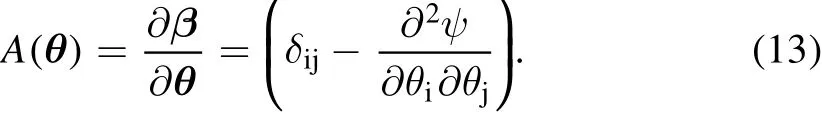
The critical line is de f ined as the curve of points in the image plane which satisfy the relation det A(θ)=0.Due to their complex mass distributions it is dif ficult to give an analytic Einstein radius for the lenses simulated in this work and we therefore follow a numerical approach.First,we use the mat pl ot lib.pypl ot.cont our module to draw the critical curve numerically(whereby the contour satis fies det A=0).The Green’s function method is then applied to calculate the enclosed area of the critical curve,Scrit.Finally,the effective Einstein radius(see Section 4.1,Meneghetti et al.2013),θE,is de fined according to the following formula,

In this work,we always report the effective Einstein radius for both the input data and the lens model reconstruction.People may use a different de finition of Einstein radius,i.e.,the“equivalent Einstein radius”,de fined as the radius of a circle(or ellipse,depending on whether the lens is circularly or elliptically symmetric)within which the average convergence is 1.For simple axis-symmetric lenses,those two de finitions of Einstein radius give the same result.

We use the mass-weighted density slope(Dutton &Treu 2014)to measure the average density slope,〈γ′〉,over a certain radial range.The global density slope in the context of strong lensing is de fined as

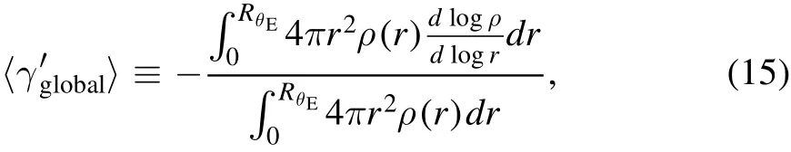
whereρ(r)is the density at radiusrand RθEis the physical size of the Einstein radius.The local density slope measures the mean density slope near the Einstein radius,which is de fined similarly as

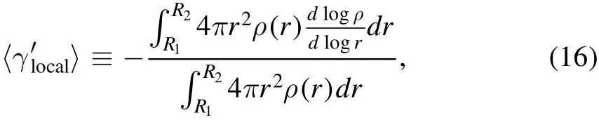
whereR1andR2are the inner and outer radius of the annulus,respectively,which encloses the extended lensed arc.Based on the true mass pro file of the mock lenses,we calculate the“global”and“l(fā)ocal”density slopes with the above equations to represent the true slope value of our mock data.These slope values are compared with the one reconstructed by lens modeling under the assumption of the EPL+shear mass model in Section 4.

2.2.Lensing Degeneracy

The SPT,which describes an intrinsic degeneracy in lens modeling,shows that different lens mass models can produce almost the same lensing observable by adjusting the lens mass and source light in a covariant fashion (Schneider&Sluse 2014).The well-known MST(Falco et al.1985,a special case of SPT)requires the source size5Strictly speaking,the change of source size is a direct result of rescaling the entire source-plane coordinates from(xs,ys)to(λ×xs,λ×ys).,re,and lens convergence field,κ,to be transformed according to

and

which keeps the lensed images invariant except for the time delay and magni fication.The relative time delay value,ΔtAB,between pairwise lensed images A and B changes according to,

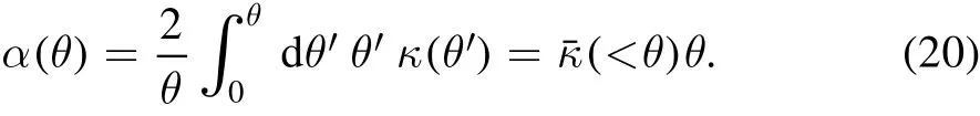
Lens modeling constrains the de flector’s mass distribution by fitting to the lensed emission,which depends upon the de flection angle field in the extended arc region.For an azimuthally symmetric lens,the de flection angles are related to the mean enclosed convergence withinθ(κˉ(＜θ))via

Suppose we have a de flector with a true mass distributionκtrue.All of the mass-sheet transformed solutions ofκtrue,which we can de fine as

provide equally good fits to the image-based lens modeling because of the MST.When we take the EPL mass model for lens modeling,the mismatch betweenκtrueand the EPL model can often be compensated by a“pseudo internal mass sheet”6We call it the“pseudo”internal mass-sheet because it does not relate to any physical mass structure.It purely originates from the mass distribution mismatch between the ideal EPL model and real lenses.(1-λpseudo).More speci fically,the transformed mass distribution κ′= λpseudo× κtrue+(1 -λpseudo) can often closely approximate an EPL model in terms of the de flection angle field(orκˉ(＜θ))near the Einstein ring.The selection of the EPL functional form therefore drives the lens model to infer the de flector’s mass distribution as an EPL approximatingκ′.

Following the discussion in Xu et al.(2016);Schneider&Sluse(2013),the speci fic value ofλpseudocan be derived analytically.We use an annular region between 0.8 and 1.2 times the Einstein radius to represent the extended-arc region.7We have also tried a different radial range:[0.5×θE,1.5×θE].Although the speci ficλpseudo value calculated from Equation(24)varies slightly,the main results in this work remain unchanged.The average density slope(s)and curvature(ξ)within the annular region([θ1,θ2])are de fined as

To summarize,the mismatch between the EPL model and the de flector’s true mass pro file could potentially bias the lens model results via lensing degeneracies.We note that,even though we only explicitly show how the MST biases the lens modeling here for clarity;the SPT,which is a generalized version of the MST,works in a similar fashion.

2.3.JAM Method

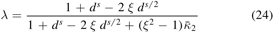
The JAM method decomposes the total mass of each galaxy into two components:a dark matter halo and a visible galaxy.The mass pro file of the dark matter halo is described by the gNFW model(Cappellari et al.2013)as

whereρsis the characteristic density,rsis the scale radius andγ controls the central density slope of the dark matter halo.For γ=1,the gNFW model reduces to the well known NFW pro file(Navarro et al.1996).For the visible galaxy,the JAM method utilized the Multiple Gaussian Expansion(MGE,Cappellari 2002)to fit the SDSSr-band image such that

whereLkis the total luminosity of thekth Gaussian component.σkandqkare the dispersion and projected axis ratio of thekth Gaussian component andNthe total number of Gaussian components used in fitting.The brightness distribution of galaxies given by MGE fitting can be transformed into the mass distribution of galaxy components by assuming a constant mass to light ratio.

Given a set of model parameters(e.g.,gNFW parameters,MGE parameters,mass to light ratio,etc.)one can derive the total mass distribution of galaxies and predict the second moment of the velocity distribution that is observed via the Jeans Anisotropic model(Cappellari 2008).Using the ensemble MCMC sampler emcee(Foreman-Mackey et al.2013)one can find the model solution which best fits the observed second moment map deduced from the MaNGA IFU data(Li et al.2018a).

2.4.Mock Lens Generation

We generate mock lenses using the surface mass density maps of ETGs in the SDSS-MaNGA project,which are derived by Li et al.(2019)with the JAM method.The redshifts of ETGs in MaNGA are from～0.02 to～0.1(median value～0.06),whereas the typical redshift of the SLACS lens galaxies(which are also ETGs)is～0.2.If the internal structure of ETGs has a dramatic evolution from redshift～0.2 to～0.02,using MaNGA ETGs to represent SLACS lenses would be unreasonable.Fortunately,results from numerical simulations(Wang et al.2019)and observations(Koopmans et al.2006,2009;Ruff et al.2011;Sonnenfeld et al.2013;Li et al.2018b;Chen et al.2019)indicate that no obvious redshift evolution exists fromz=1 toz=0 and we therefore anticipate that our mock lenses will be representative of SLACS lenses.To ensure our mock lenses are most similar to those in the SLACS sample,we“move”a MaNGA ETG to redshift 0.2 and suppose that it acts as a strong lens with a background source at redshift 0.6.We require that the final MaNGA ETGs used to generate the mock lenses meet the following criteria:

1.The Einstein radius of the mock lenses ranges between 0 6 and 2 0.

2.The luminosity-weighted velocity dispersion within the half-light radius of each ETG is larger than 150 km s-1.

3.The Sérsic index(Sérsic 1963)is larger than 3 to ensure the galaxy is an ETG.

4.The results of JAM modeling are labeled as Grade-A in Li et al.(2018a),to ensure that the dynamical reconstruction is reliable.

We utilize the surface mass density map(Σ)used in Li et al.(2019)divided by the critical density of the lens system(Σcrit)to compute the convergence

whereΣcritis given by

We then apply a fast Fourier transform algorithm toκto calculate the de flection angle map employing Equation(11).To reduce the numerical errors of the de flection angle calculation,we apply the following scheme:

1.The de flection angle is calculated numerically on an oversampled grid of resolution 2×2,where the average is taken to give the de flection angle on the coarser native image grid(0.05″/pixel).

2.To avoid the boundary effect shown in Van de Vyvere et al.(2020),we perform the Fourier transform on a grid of size 40″×40″whose half-width is at least 10 times larger than the typical Einstein radius8We demonstrate the necessity of taking a larger convergence map size to robustly estimate the de flection angle in Appendix B..

3.When Equation(11)is used for numerical convolution operation,the size of the kernel is twice the size of the de flection angle map.

The de flection angle map derived from the above method is utilized to generate mock lenses.The ideal lensed image,Iideal(θ),can be expressed as

whereIs(β)is the brightness distribution of the source galaxy in the source-plane.In this work,we use asingleSérsic component to representIs.The expression of a Sérsic pro file is wherereis the half-light radius,Ieis the brightness atre,nis the Sérsic index andbnis a coef ficient that only depends onn.We can introduce ellipticity into Equation(30)via the coordinate transformation described by Equation(4).To create our 50 mock lenses,we always assumere=0.15″,n=1.0 and axis ratioq=0.7(Newton et al.2011).The position(xs,ys)of the source galaxy is drawn from a Gaussian distribution with mean 0″and a standard deviation 0 1,and the position angle is uniformly selected between 0°and 180°.By utilizing this set of parameters,the final lensed images we generate usually have extended arc structures.The constraining power provided by lensing is related to the geometry con figuration of the lens system (cusp,fold,two images,Einstein cross)and the extended arc can provide more information on a de flector’s mass distribution,which helps to reduce systematic errors in the final modeling result(Tagore et al.2018).Since this work focuses on evaluating the systematic errors of galaxy-galaxy lens modeling under the EPL assumption,we choose to model a variety of lensing con figurations and do not speci fically assess the in fluence of a given lensing con figuration on our modeling results.

To simulate observational effects,the image pixel size is set to 0 05(HST-quality).The ideal lensed image derived by Equation(29)is convolved with a Gaussian Point-Spread Function(PSF,standard deviation:0 05).We assume a sky background of 0.1 counts s-1and an exposure time of 840 s.Background noise from the skylight and Poisson noise from the target source is also added to mock images.We manually adjust the brightnessIeof the source galaxy to ensure that the peak signal-to-noise ratio of each lens in our final sample is～50,which roughly corresponds to the highest signal-to-noise observations in the SLACS project(Bolton et al.2008a).

To compute true time-delay values of our mock lenses at a given set of image positions,we need true lens potential values ψ.We use Equation(12)to calculate the lens potential map from theκmap and apply the strategy described previously to reduce the numerical error on the fast Fourier transform.The lens potential at any position on the lens plane can then be obtained via interpolation.

Figure 1 shows the sample of 50 lenses that we simulated,which we refer to hereafter as the“MaNGA lenses”for short.All our lensing images have extended arc structures,which make them a good probe of the underlying mass distribution.The green circles mark the lensed positions of the center of the source galaxies.The time-delay values between these positions are calculated and used when we test the measurement ofH0.

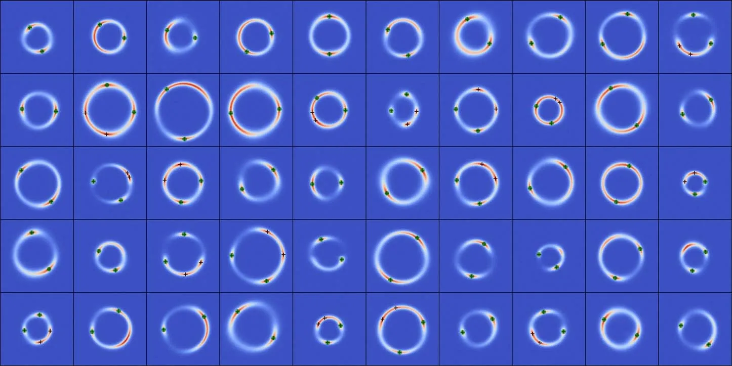
Figure 1.Images of 50“MaNGA lenses”.For each lens,locations marked by the black crosses represent the lensed positions of the source center;the points marked by the green circle are used to calculate the excess time-delay between different images as shown in Figure 16.The scale-bars mark the angular scale of 1 arcsecond.

Figure 2 depicts the relationship between the Einstein radius(measured from Equation(14))and the half-light radius of the MaNGA lenses(measured from the Sérsic fit,left panel),and the probability density distribution of their Einstein mass(right panel).For comparison,we also show the values of lenses in SLACS(in orange).One can find that the distribution of properties of our mocks and those of lenses from SLACS are quite similar.

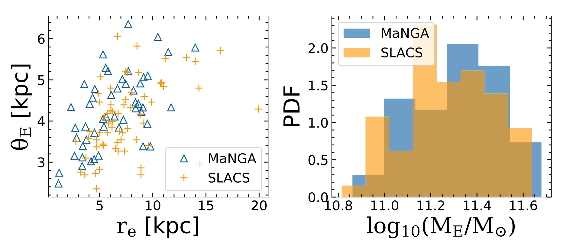
Figure 2.The left panel features the dependence of the Einstein radius on the half-light radius of the lens galaxy.Each data point corresponds to a lens system,blue represents“MaNGA lenses”and orange represents SLACS lenses.On the right panel,the blue histogram shows the Einstein mass distribution of“MaNGA lenses”and the orange histogram represents the distribution of SLACS samples.

3.Modeling Methodology

We use Py Aut o Lens(Nightingale et al.2021b)9The Py Aut o Lens software is open-source and available from https://github.com/Jammy2211/PyAutoLens.to model the simulated“MaNGA lenses”,which is described in Nightingale et al.(2018,N18 hereafter)and builds on the works of Warren&Dye(2003),Suyu et al.(2006),Nightingale&Dye(2015).Py Aut o Lens uses an empirical Bayes framework and a technique called nonlinear search chaining to compose pipelines which break the lens modeling procedure into a series of simpler model-fits.This allows a user to begin modeling a system with a simple lens model(e.g.,an isothermal mass pro file and a Sérsic source)and,via a sequence of nonlinear searches,gradually increase the model complexity,so as to eventually fit the desired more complex lens model(in this work,an EPL+shear using a pixelized source reconstruction).Non-linear search chaining is implemented in Py Aut oLens via the probabilistic programming language Py Aut o Fi t10https://github.com/rhayes777/PyAutoFitand it provides three main advantages for lens modeling:

1.For complex lens models,the nonlinear search may not be able to sample parameter space suf ficiently well to find the global maximum-likelihood solution and may instead infer an inaccurate local maximum.Fitting simpler lens models in early searches helps mitigate this,since the results of fitting a simple model can guide the choice of prior for the more complex models fitted by subsequent nonlinear searches.By providing the nonlinear search a better initialization of where to search the parameter space,one can therefore reduce the risk of inferring a local maximum.This allows us to achieve fully automated lens modeling in this work.

2.The settings of Py Aut oLens and the nonlinear search are customized to give fast and ef ficient model-fits in early stages of a pipeline(where a precise quanti fication of the model parameters and errors is not required)and perform a more thorough analysis later on(where a precise estimate of the lens model parameters and errors is desired).

3.In addition to the results of the lens model itself,other results of the model-fit are also passed to the fits performed later on.For example,we use Py Aut oLens's“hyper-mode”,which fully adapts the model to the characteristics of the imaging data that are being fitted by passing the model-image of the lensed source galaxy inferred by earlier fits to later fits.

We use a single Sérsic pro file to represent the brightness of the source galaxy when we simulate the“MaNGA lenses”.We can therefore in principle“perfectly”represent the source’s light using a Sérsic source model.However,for real strong lens observations,the brightness distribution of the source is often irregular and complex,which necessitates the use of pixelized source models(Nightingale et al.2018).To ensure our results can generalize to observations of real strong lenses,we therefore use a pixelized source reconstruction to fit the lens model,even though a Sérsic source would suf fice.We use the adaptive brightness pixelization and regularization scheme provided by Py Aut oLens to do this.The adaptive pixelization congregates source-pixels to the regions where the source is located,effectively improving the resolution of the source reconstruction.Adaptive regularization makes it so that Py Aut o Lens can reduce the regularization strength of the source in its central regions relative to its outskirts,which is important for reconstructing sources with compact or clumpy structures.

To perform model-fitting via nonlinear search chaining,we use the“SLaM”(Source,Light,and Mass)pipelines distributed with Py Aut oLens to model our“MaNGA lenses”.In brief,our lens modeling pipeline divides the lens modeling process into three steps:

1.The mass distribution of the lens is modeled by a singular isothermal ellipsoid+shear.The brightness distribution of the source is modeled by a Sérsic component.The lens modeling results of this step tell us the approximate mass distribution of the lens,which is next used to initialize the pixelized source model.

2.Based on the results of the mass model in step(i),the pixelized source model is fitted.

3.Based on the optimal pixelized source model obtained in step(ii),fit the lens mass with the EPL+Shear model.

This pipeline therefore finishes by fitting the EPL+shear model,on which the majority of our results are based.During the lens modeling,we require a feasible lens mass solution to ful fill the following condition:after tracing positions marked by black crosses in Figure 1 back to the source plane,those points should be located within a small range(a circle with a radius of 0 3).11Although we do not explicitly use the position of the selected lensed images to constrain the lens mass model(i.e.,integrate the position constraints into the Gaussian-form likelihood function),we found that after tracing the selected lensed images shown in Figure 1(marked by black crosses)back to the source plane(using the best-fit lens model based on the extended arc),the distance between them does not exceed 0.05″.Therefore,we expect that the extended arc has already ef ficiently constrained the lens mass model,and the positions of the counter images will not provide too much extra contribution.

This trick can improve the modeling speed and avoid solutions with non-physical sources.For a more detailed overview of the modeling procedure,we refer to the flow chart illustrated in Figure 3.12For more speci fic prior-passing con figurations,see the online material:https://github.com/Jammy2211/autolens_workspace.

The goal of the paper is to study the systematic errors induced by the EPL mass model when the true mass distribution of a lens system is more complex.Since the more flexible pixelized source model can“absorb”some of the residual signals due to the mass model mismatch,it is important to check whether this affects the lens mass parameters we estimate.Therefore we performed an additional set of model fits whose source light is represented by a parametric Sérsic.The lens mass parameters determined by model fits with the parametric source model are statistically consistent with those derived by assuming the pixelized source model,hence we only report the results of the pixelized source model.

4.Results and Discussion

This section presents the lens modeling results of our mock“MaNGA lenses”under the assumption of the EPL+shear lens model.Section 4.1 lists the reconstruction results of the lens mass model,including the measurement of Einstein radius(Section 4.1.1),shear(Section 4.1.2)and density slope(Section 4.1.3).Section 4.2 describes how the source reconstruction is in fluenced by the EPL assumption.We show the anatomy of individual lens systems for a typical case and an outlier in Sections 4.2.1 and 4.2.2,respectively.The statistical results of source reconstructions are presented in Section 4.2.3.We will discuss how the EPL mass assumption affects the estimation of time-delays andH0in Section 4.3.

4.1.Mass Model Reconstruction

In this section,we discuss the systematic errors caused by assuming the EPL+shear mass model for measurements of the Einstein radius(Section 4.1.1),shear(Section 4.1.2)and inner density slope(Section 4.1.3).

4.1.1.Einstein Radius

Figure 4 displays the inferred Einstein radius of our 50“MaNGA lenses”under the assumption of EPL+shear mass model.We find that the relative systematic error of the model is only 0.05%±0.17%(68%con fidence level),indicating that the estimation of Einstein radius is unbiased.Given that the magnitude of the statistical error is only of order 0.01%and its error bar is almost invisible,we only report the typical value of the statistical error in the legend of the right panel.Summing both statistical and systematic errors in quadrature,our results indicate that lensing can determine the Einstein radius with an accuracy of～0.1%.

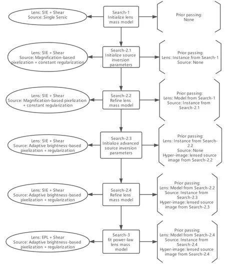
Figure 3.This figure illustrates the modeling process using the advanced pixelized source model provided by Py Aut o Lens.The middle box shows the purpose of the current nonlinear search.The model component of the current nonlinear search is recorded in the left ellipse.The bracket on the right shows the prior transfer of the current nonlinear search,where“instance”represents that the parameters of the model inherit the best-fit results of previous nonlinear searches,and stay fixed during modeling;while“Model”is similar to“instance”,but inherits parameters in the Gaussian prior way.

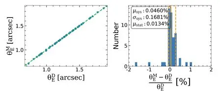
Figure 4.The left panel compares the model value of Einstein radiiwith the ground truth onesde fined by Equation(14)).Each data point represents the model reconstruction of a lens system;a data point lies on the green dashed line if the model value matches the true value perfectly.Since the statistical error on the Einstein radius is small(only of order 0.01%),we do not include the error bar for each data point on the left panel,and only present the median of the relative statistical error(μstat)in the legend of the right panel.The right panel depicts the number distribution of relative systematic error.The orange solid vertical line shows the median value of the relative systematic error distribution,and the two orange dashed vertical lines mark the 68%con fidence interval([16%,84%]percentile).We show the median(μsys)and dispersion(σsys)(i.e.,the standard deviation)of the systematic error in the legend.

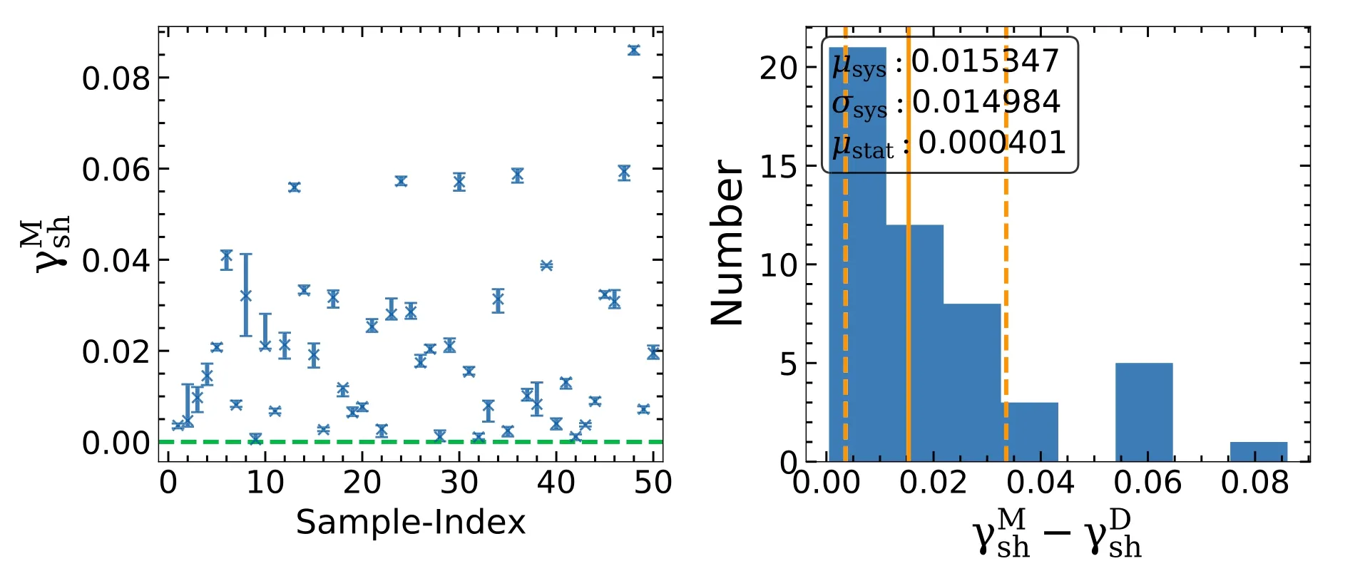
Figure 5.Similar to Figure 4.The shear strength reconstructed by the lens model is compared with the true value.The error bars represent the 3σlimit of each lens.Given that we do not include the external shear component when simulating mock data,the ground truth value of the shear strength is zerowhich is marked by the green dashed line.The right panel shows the distribution of the absolute systematic error.

As a demonstration,we consider a constraint on the post-Newtonian gravity parameterγppn,following the method of Bolton et al.(2006c),Schwab et al.(2010),Cao et al.(2017),Collett et al.(2018),Yang et al.(2020).This compares the mass of galaxies from lensing and stellar dynamics

Assuming that the measurements of stellar dynamics are errorfree,such that the only source of bias is from lensing,our～0.1%relative error on Einstein radius translates into an error of～0.004 onγppn(see Appendix C).This is an order of magnitude smaller than current measurement uncertainty(γppn=0.97±0.09,Collett et al.2018).Therefore,use of the EPL mass model does not currently limit this test of gravity.

4.1.2.Shear

The distribution of shear strength measured for each lens model is displayed in Figure 5.Although we did not add an external shear term when generating mock data,we have to include a shear component when doing lens modeling,otherwise we get a bad image fit with signi ficant residuals.The median inferred shear magnitude for our 50“MaNGA lenses”is 0.0153 and the standard deviation is 0.0150.Recall that when we simulated the mock lenses,the surface mass distribution of their stellar components was given by the MGE model which did not possess homoeoidal elliptical symmetry.13Each elliptical Gaussian component in MGE shares a common center and position angle,but the axis-ratio is allowed to be different.For the dark matter the gNFW model was applied,which is circularly symmetric.The total surface mass density of simulated lenses therefore does not satisfy elliptical-symmetry and the EPL lens model by itself is unable to describe this departure from elliptical symmetry.However,the shear term can mimic the effect of deviating from elliptical-symmetry to a first-order approximation (Keeton et al.1997).This is illustrated more clearly in Figure 6.For the mock lens depicted in Figure 6,the critical line of the MGE+gNFW simulated mass distribution has a“boxy”shape(black line)because it does not satisfy elliptical symmetry.The EPL model by itself gives a critical line(yellow dotted line)with an elliptical shape that closely traces the black line,but is unable to trace it perfectly.By including a shear,the EPL+shear model’s critical line(red dashed line)more closely approximates the true pro file’s“boxy”shape.Therefore,the shear detected in this work is an internal shear caused by theκfield of the lens system itself that does not satisfy the elliptical-symmetry,rather than an external shear caused by line of sight structures.

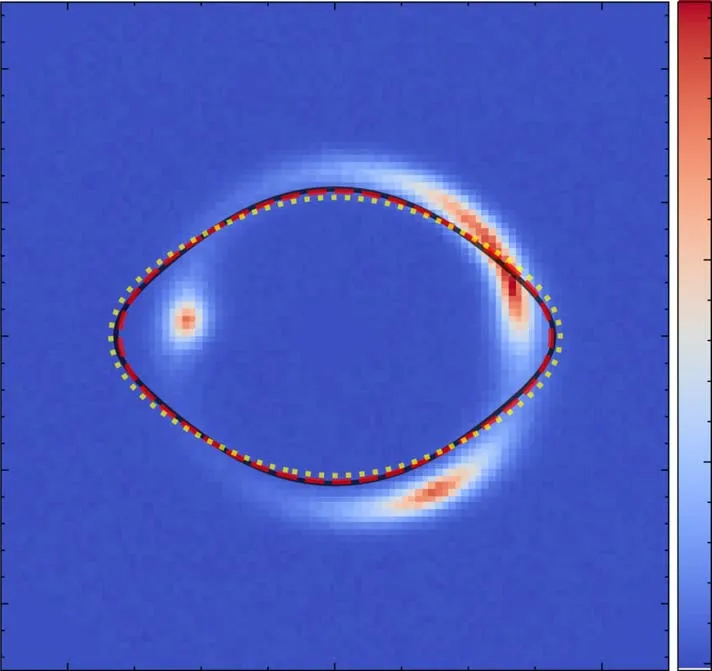
Figure 6.The best-fit lens model of system“3024_9039-1902”.The black line represents the true critical line of the mock data.The yellow dotted line marks the critical line given only by the EPL model,while the red dashed line is the critical line predicted by the EPL+shear model.

Cosmic shear can be used to infer the mass perturbations along the line of sight,making it an important probe of the large-scale structure of the universe.Birrer et al.(2017,2018)proposed using strong gravitational lens systems with extended ring structures to measure cosmic shear,where a combination of this measurement with weak lensing can illuminate the different systematic errors between the two methods.Our results here show that when using strong gravitational lenses to measure the cosmic shear,it may be important to ensure the method is not subject to systematic errors induced by the lens not possessing elliptical-symmetry.

4.1.3.Density Slope

Our lens models accurately recover the global density slope,de fined as the mass-weighted density slope within the Einstein radius(Equation(15)).Averaging across our mock sample,the inferred global density slope is smaller than the input value by only 2.5%,with a root-mean-square scatter of 3.4%(top panel of Figure 7).However,the local density slope at the Einstein radius,de fined as the mass-weighted density slope within the radial interval[0.8×θE,1.2×θE](Equation(16))is less accurately recovered.It is underestimated(on average)by 13.3%with a scatter of 11.2%(bottom panel of Figure 7).

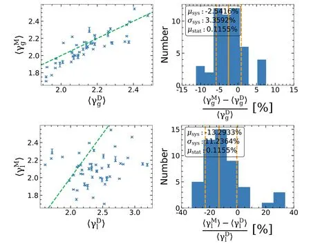
Figure 7.Top panel:Reconstruction of the de flector’s“global density slope”〈γg〉within the Einstein radius.Error bars in the left panel show 3σlimits.Bottom panel:Reconstruction of the de flector’s local density slope〈γl〉near the Einstein radius.Green dashed lines indicate the 1:1 relation.

It may seem counter-intuitive that we measure the density slope better for the whole lens than at the speci fic radius of the source flux,and similar results have also been observed in O’Riordan et al.(2020).Following Kochanek(2020),we had expected a measurement of global density slope to be just an extrapolation of the local mass distribution inferred by lensing with the EPL functional form.Our result is explained by the mismatch between the ideal EPL model and real lenses.Pure image-based lens modeling under the EPL assumption will infer the de flector’s mass pro file as approximately the true mass pro file after an SPT transform,because this transformed mass pro file more closely follows the functional form of the EPL model in terms of the de flection angle field(or approximately average convergence within radiusθ,κˉ(＜θ),see Equation(20))near the Einstein ring.

This mismatch directly leads to the 11“outliers”in our modeling results,whose physical parameters such as the source size and the lens density slope are signi ficantly misestimated.Furthermore,we find the modeling results of nine outliers can be approximately understood via the classical MST,a special case of the SPT.As an example,we present the anatomy of a typical outlier(“3485_8153-3701”)in Figure 8,whose local density slope is signi ficantly misestimated.The left panel of Figure 8 features the radial density pro fileκˉ(＜θ)of the de flector.The black solid line shows the de flector’s true mass pro file while the red solid line represents that inferred by the best-fit EPL+shear lens model.Clearly,the reconstructed density pro file mismatches the input one although the overall fitting of the image is good.For this system,the mass distribution mismatch between the ideal EPL model and“MaNGA mock lenses”can be compensated by a mass-sheet transform ofk′=λκ+ (1 -λ).We apply the MST to the de flector’s true density pro file(black line)and show the resulting pro files using orange and green lines,where theλfor the orange line is derived using Equation(24)and theλfor the green line iswhereare the source size of the model and the ground truth value,respectively(see more discussion in Section 4.2).One finds that both lines are nearly coincident with the one inferred by the lens model(red line)near the Einstein ring(marked by the shaded gray),and by de finition,the mass pro file of both green and orange lines can produce the same lensed image as that of the input mass distribution.Therefore,the mass distribution mismatch between the EPL model and our“MaNGA mock lenses”drives our pure image-based lens model pipeline to approach a biased solution,i.e.,an“MST solution”of the de flector’s true mass distribution.To demonstrate how the above effect directly affects the inferred local density slope,we show theκpro file of this lens system in the right panel of Figure 8.The local density slope of the de flector(the black solid line)near the Einstein ring is substantially different from the value inferred by the lens model(the red solid line).

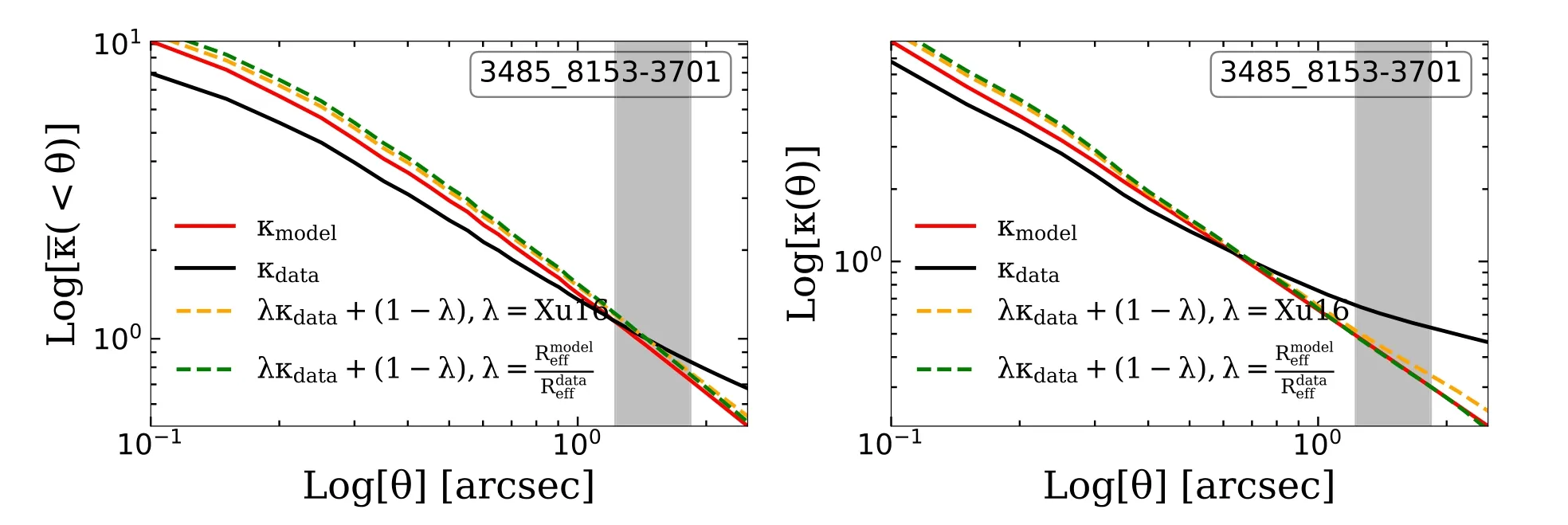
Figure 8.The convergence pro file of the lens system“3485_8153-3701”whose lens model bias due to the oversimpli fied EPL mass model can be understood via the MST.Left:the red solid line represents the radial pro file of the average convergence within certain radii(κˉ(＜θ))predicted by the lens modeling.The intrinsic average convergence pro file of data is shown with the black solid line.Other lines are mass-sheet transformed solutions of the black line.The correspondingλfactor of MST for the orange dashed line(λ=1.42)is given by Equation(24),which makes its de flection angle field most similar to the power-law functional form in the vicinity of the Einstein ring marked by the shaded gray.Theλfactor for the green dashed line(λ=1.49)is the ratio of the model’s source size to the input true value.Right:the(non-averaged)radial density pro fileκ,lines with different styles correspond one-to-one to the left panel.

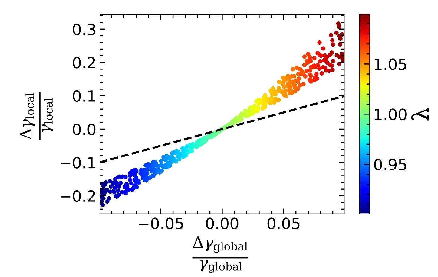
Figure 9.Each data point corresponds to an ideal spherical power-law lens,with the Einstein radius set to 1 0,and density slope ranging from 1.9 to 2.3.An MST with aλvalue in the range from 0.9 to 1.1(shown with the color bar)is exerted on each lens.We compare the relative change of the de flector’s local/global density slope before and after doing the MST.The black dashed line marks the relation in which the relative change of local density slope is equal to the global one.

The measurement of the global density slope is in fluenced by a similar effect.However,the global density slope is less impacted by the MST(or SPT).In other words,when we use an MST to rescale the de flector’s true mass pro file with Equation(17),the relative change of the local density slope is larger than the global density slope.We demonstrate this point via a toy model in Figure 9.We find the relative change of local density slope reaches beyond 30%in some cases,but the relative change of global density slope is still below 10%.

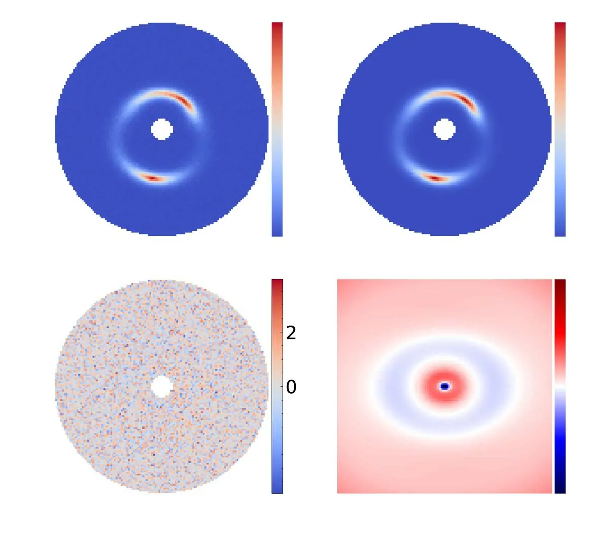
Figure 10.The lens modeling result of a typical system“1344_8263-9102”,which is fit well by an EPL+shear mass model.Top-left:the image of mock data I data;Top-right:the reconstruction of lens modeling I model.Bottom-left:the normalized residual map of the best-fit model,de fined as(I data-I model)/I noise,where I noise is the noise map of the mock data;Bottom-right:the relative error map between the convergence map of the model(κmodel)and the ground truth value(κdata),which is de fined asκdata/κmodel-1(in accordance with Enzi et al.2020).Contours mark the lensed image of the mock data.

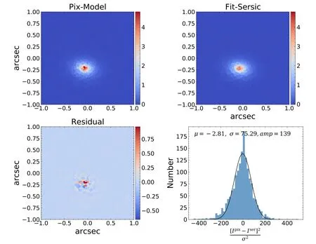
Figure 11.The source reconstruction of the MaNGA lens“1344_8263-9102”.Top-left:the pixelized source reconstruction corresponding to the best-f it lens model.Top-right:the best-f it Sérsic model to the pixelized source reconstruction,displayed using the same Voronoipixelsasused in the source reconstruction.Bottom-left:t heresidual map of thebestSérsicfi t,i.e.,top-leftimageminustop-rightimage.Bottom-right:thebluehistogramshowsthe number distributionofthenormalized residual(?seeEquation(32))ofthebestSérsicf it.AGaussianf ittothisdistributionisshownwiththeblackline,and thecorrespondingbest-fitmean(μ),standard deviation(σ)and amplitude value(amp)are reported in the text label.This distribution hasatail with large normalized residual values(～100),because the source uncertainties are typically underestimated in the outskirts of the source.

Overall,the global density slope recovered by the EPL model is suf ficiently accurate for current tests of galaxy evolution(Wang et al.2019,A.Etherington et al.2021,in preparation).Accurately measuring local density slope,however,may require a form of mass distribution that better represents the target lens(to avoid the mass distribution mismatch discussed above),or combining with additional observables to provide extra constraints that break the degeneracy(Koopmans et al.2006,2009;Shajib et al.2020;Y?ld?r?m et al.2020).

Note that stellar dynamics constrains the three-dimensional mass distribution,while lensing measures the projected twodimensional mass distribution.To compare these two independent mass estimators,one can project the three-dimensional mass distribution given by stellar dynamics to get the projected(two-dimensional)mass distribution or deproject the twodimensional mass distribution inferred by lensing to infer the three-dimensional distribution.Here,we choose the latter,converting the two-dimensional density slope inferred by lensing to the three-dimensional density slope—which in the case of a power-law density pro file means adding one to the power-law exponent.We report our findings in terms of the three-dimensional density slope for consistency with previous work(He et al.2020b;Shajib et al.2020;Newman et al.2013;Dye et al.2008).

4.2.Source Morphology

Gravitational lenses can be utilized as cosmic telescopes to study the structure of their highly magni fied source galaxies.An important question is whether the lens modeling process reconstructs the source’s morphology accurately and with high fidelity?Approaches such as the pixelized source reconstructions used in this work can reliably recover the structure of the source when the lens mass model is correct(Warren&Dye 2003;Suyu et al.2006;Tagore& Keeton 2014;Nightingale&Dye 2015;Nightingale et al.2018).However,for real lenses the mass model will not perfectly describe the lens’s true underlying mass distribution and this mismatch could potentially bias the source reconstruction,in particular via the way of the SPT.In this section,we rely on our“MaNGA lenses”test suite to evaluate systematic errors of the source reconstruction caused by the oversimpli fied EPL mass model.

4.2.1.Typical case:“1344_8263-9102”

Our lens models capture the overall structure of almost all lens systems well.The fit to a typical lens-plane image(using an EPL+shear mass model and pixelized source)is displayed in Figure 10.The normalized residuals for this fit,which are shown in the bottom left panel,are almost within the＜3σlimit,indicating a good lens model.Furthermore,the inferred convergence broadly agrees with the input values in regions near strongly lensed images,as shown in the bottom right panel.

The source morphology is also typically recovered well.To compare the pixelized model inferred by Py Aut oLens to the input Sérsic model,we fit the model source-plane image with another Sérsic,by minimizing the followingχ2function

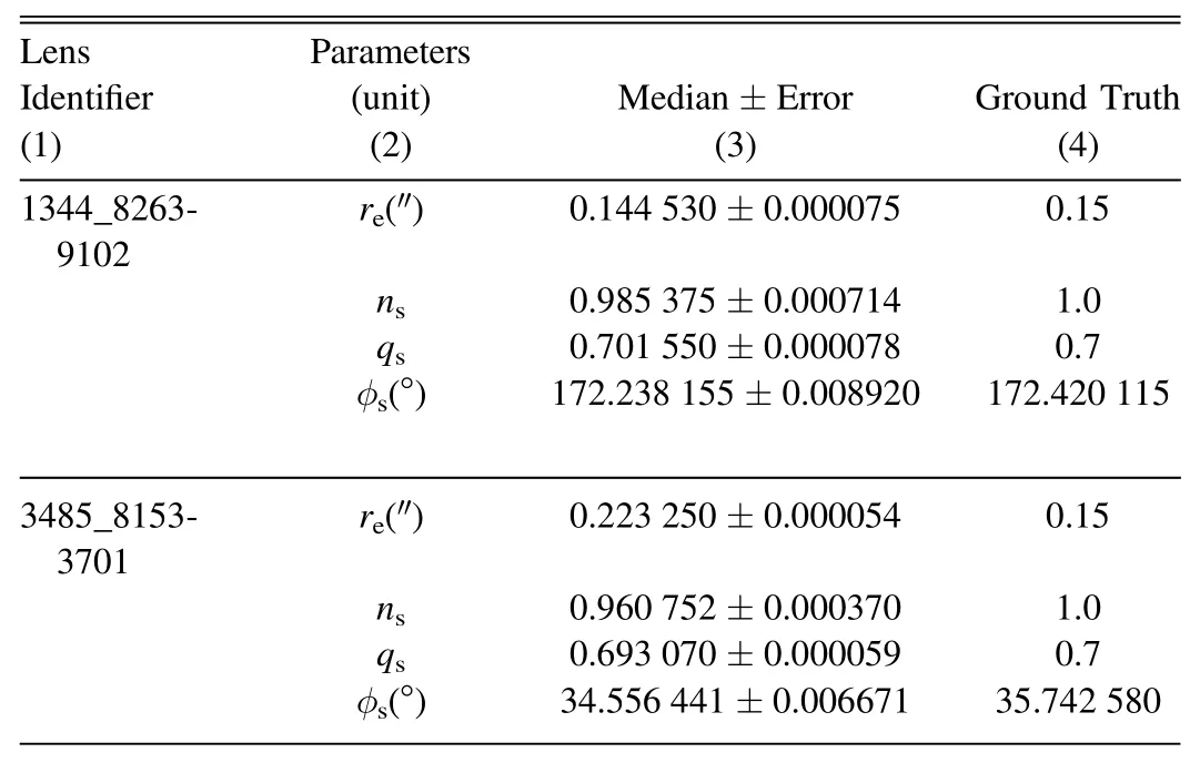
Table 1 A Sérsic Model is used to Fit the Pixelized Source-reconstruction of our Mock“MaNGA Lenses”

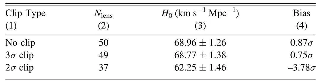
Table 2H0 Constraints given by the Joint Analysis

Two possibilities might explain why systematic errors are larger than statistical error.First,the model is over-constrained because we assume an EPL mass model with insuf ficient complexity to represent our mock“MaNGA lenses”.Any restricted mass model drives a precise but inaccurate source reconstruction(Kochanek 2020).Second,a recent study has demonstrated that the advanced pixelized source modeling provided by Pyaut ol ens leads to stronger discretization noise compared with other“traditional”methods(e.g.,Suyu et al.2006;Vegetti&Koopmans 2009)without“random pixelization”features(see Nightingale&Dye 2015),which may also weakly bias the source reconstruction.A“stochastic likelihood cap”can mitigate this kind of bias(Etherington et al.in prep.).

4.2.2.Outliers

Except for the typical system described in Section 4.2.1,we notice that there are some“outliers”in our modeling results.Although the model still roughly recovers the source’s shape(axis-ratio,position angle),the source’s size is signi ficantly misestimated.To make sure these“outliers”are not caused by bad lens modeling,we visually inspect the normalized residual map14https://github.com/caoxiaoyue/Sim_MaNGA_lens/tree/main/best_fit_result_subplot(bottom-left panel in Figure 10)and the source reconstruction image15https://github.com/caoxiaoyue/Sim_MaNGA_lens/tree/main/src_fit_image(top-right panel in Figure 11)of each lens system.We find the normalized residuals are typically within the～3σlimit and that every source reconstruction appears physical,i.e.,it does not show the unphysical structure that is demonstrated in Maresca et al.(2021).Therefore,our lens modeling results are fairly good.

The cause of outliers is essentially due to the mismatch between the ideal EPL model and the“true”mass distributions of our mock lenses,which results in a biased source reconstruction via the SPT.Figure 12 shows a representative outlier(“3485_8153-3701”),whose modeling bias can be quantitativelyunderstood via the MST(a special case of the SPT).Recall the mass pro file of the lens system“3485_8153-3701”we presented in Figure 8,in which the green dashed line represents the masssheet transformed solution of the de flector’s true mass pro file.The correspondingλfactor is given by the ratio of the source size inferred by the lens model to the input true value.The coincidence of the green dashed,orange dashed and red solid line in the shaded gray region indicates that the degeneracy in this system can be understood well via the MST.More speci fically,theλfactor corresponding to the orange dashed line is 1.42,which is consistent with the model’s source size being overestimated by a factor of 1.49(recall Equations(17)and(18)).

4.2.3.Population Statistics

For all 50“MaNGA lenses”simulated in this work,we carry out the analysis described in Section 4.2.1.The global morphology properties of our pixelized source reconstructions are statistically summarized in Figure 13.We find that the lens models accurately recover the sources’position angles(φs,absolute systematic errors with the median value of-0°.0368,and standard deviation of 1°.2452)and axis-ratio(qs,absolute systematic errors with the median value of-0.0101 and standard deviation 0.0088);However,the size of the source(rs)and its Sérsic index(ns)are underestimated by 6.77%and 3.92%on average respectively.Combining the result of bothrsandns,sources reconstructed by the lens model are slightly more compact than their true appearance.

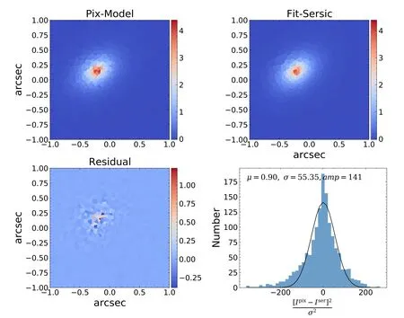
Figure 12.Similar to Figure 11,the source reconstruction of the MaNGA lens“3485_8153-3701”.

Our algorithm tends to reconstruct an overly compact source galaxy on average because the input mass distributions are cuspier than can be described by an EPL model(Figure 14).This mismatch leads to～7%underestimation of the convergence near the Einstein ring,and～7%underestimation of the source size via the SPT.16When lensing degeneracies are manifested as the MST,the underestimation of the convergence near the Einstein radius is indirectly related to the underestimation of the source size through theκˉ(＜θ)(see Equation(20)).Therefore,the consistent～7%number here could be just a coincidence.We find the degeneracy in most lens systems can be approximated as an MST(see Figure 15).Of our 50 mock lens systems,the sizes of 39 source galaxies are modeled within 20%of the true value,and we designate the remaining 11 systems as“outliers”.Among the“outliers”,the modeling bias in nine systems can be understood in terms of the MST(see the discussion in Section 4.2.2).The remaining two outliers re flect the more general SPT,where the difference between the model and the true value of the two-dimensional convergence map in the region of the lensed arc cannot be compensated by a uniform mass sheet,in either the radial or angular direction.We further show those two“Non-MST outliers”in Appendix D.

4.3.Time Delay and H0 Inference

For every pair of multiply lensed images(marked by green circles in Figure 1),we calculate the relative time delay de fined in Equation(8).By comparing the model value of each pairwise relative time delayΔt Mwith its true valueΔt D(Figure 16),we investigate the systematic error caused by our assumption of the EPL+shear model.We find relative time delays to be underestimated,with median relative systematic error 5%and standard deviation 18%.This underestimation is qualitatively consistent with the underestimation ofκnear the Einstein radius for most lenses in our sample(see the average trend in Figure 14),which rescales the relative time delay according to(19).Furthermore,the six lens systems whose time delay measurements are discrepant by more than 4 days17Considering the typical time-domain measurement uncertainty for current instruments is～2 days,4 days roughly corresponds to 2σerror.also suffer from signi ficantly overestimated or underestimated κat the image locations.Thus,although the EPL model can approximately describe the density pro file of the lens in a statistical sense,the density pro file of an individual lens system may still deviate signi ficantly from the EPL model,resulting in large discrepancies between the predicted and true relative time delays.

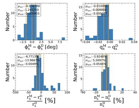
Figure 13.The top panels depict the distribution of absolute systematic errors for sources’position angle(φs)and axis-ratio(q s),with the median(μsys)and standard deviation(or dispersion,σsys)of the systematic error,and the median value of the statistical error(μstat,purely predicted by the nonlinear search sampler)overlaid on the legend.The bottom panels show the distribution of relative systematic errors for sources’effective radius(r s)and Sérsic index n s.Three orange lines mark the[16%,50%,84%]percentiles of the histograms.

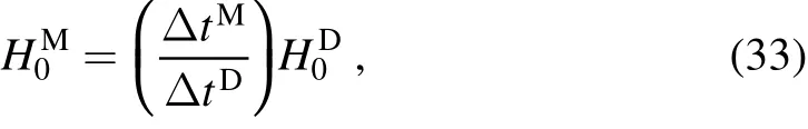
In time-delay cosmography,a biased estimation in the relative time delay between pairwise lensed images can be further interpreted as a biased estimation of Hubble constant(H0M),via the following relation(see the derivation in Appendix E)

where we assume a fiducial valuekm s-1Mpc-1.Figure 17 displays the probability density function(PDF)ofH0obtained using the inferred pairwise relative time delays of every lens system.The width of each PDF is purely governed by the statistical errors of the lens mass model.They are narrow because the over-simpli fied EPL mass model can drive a very precise but inaccurate lens mass model(Kochanek 2020).We findH0Mmeasurements randomly distributed between 40 km s-1Mpc-1and 110 km s-1Mpc-1.This result is signi ficantly less homogeneous than state-of-the-art time-delay cosmography projects.For example,the H0LICOW project measuresH0using six gravitationally lensed quasars with measured time delays,and five of them are analyzed blindly(Wong et al.2020).In their results,theH0values predicted by each lens cluster around 73.3 km s-1Mpc-1and yield statistically consistent results(see Figure 2 in Wong et al.2020),indicating that they do not underestimate statistical errors and successfully control the systematics.Systematic errors are larger in our results,because our pure image-based lens model is subject to degeneracies of a“pseudo internal mass-sheet”(see Section 2.2),induced by the mismatch between the ideal EPL model and the more complex distribution of mass in our mock“MaNGA lenses”.To reduce this systematic error and obtain an unbiasedH0measurement,velocity dispersion is crucial(Sonnenfeld 2018).

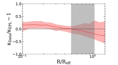
Figure 14.The residual projected density pro file is plotted as a function of radius(normalized by the effective radius of the lens’light).This shows the difference between the best-fit model’s surface density and the ground truth values.This was calculated for each of our 50 mock lenses,with the red solid line showing the median deviation between the best-fit models and the respective truths,while the red shaded region illustrates the 16th–84th percentiles of the residuals at each radius.The gray shaded region represents the 16th–84th percentiles of the distribution ofθE/R eff in our lens sample.The black dashed line represents the curve when the lens model perfectly recovers the surface density pro file that generated the data.

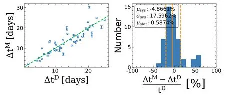
Figure 16.Reconstructed measurements of the time-delay between pairs of images of the same source,Δt M,across our mock lens sample,compared to the true value,Δt D.These are underestimated by～5%on average.

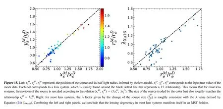
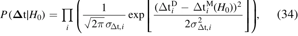
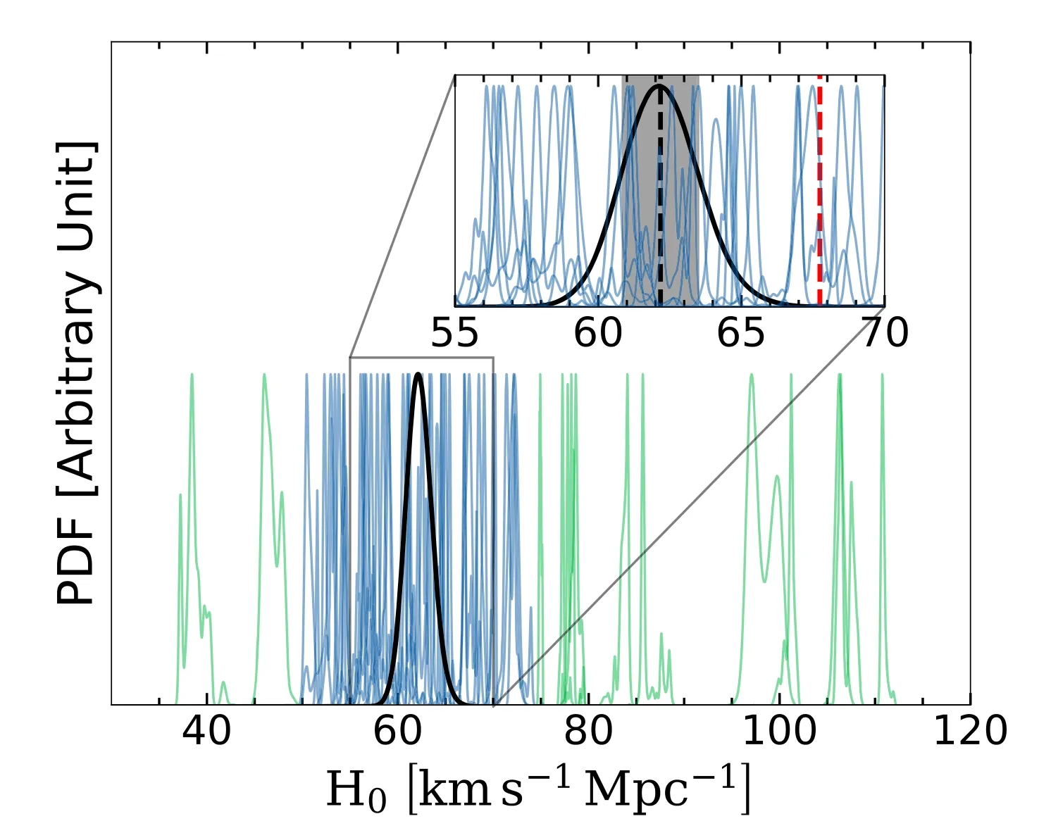
Figure17.PDFof H0 predicted by each individual lens,shown with blueand green histograms.Thewidth of each blueand green histogram ispurely governed by the statistical errors of the lens mass model.Lenses corresponding to green histograms are excluded from the joint H0 inference via the 2σclipping,to avoid the bias introduced by these extreme systems.The black histogram is the PDF of H0 constrained by a joint analysis of 37 lenses(indicated by blue histograms).We renormalize each PDFto the sameheight for better visualization.Theinset plot showsthezoomed-view around theblack histogram.Thered vertical dashed line marks theinputtrue valueofthe H0.Theblackverticaldashedlineandtheshadedgraymarkthe medianvalueand the68%con f idence interval of theblack histogram(i,e,62.3±1.3km s-1 Mpc-1)respectively;thispredictionofH0is～4σlowerthantheinputtruevalue(67.7 kms-1 Mpc-1).

We further explore using multiple lens systems to jointly constrainH0.We write the joint likelihood as where the subscriptiruns over all lens systems.We assume uncertainty on time delay measurementsσΔt,i=2 days,which is typical for recent time-domain observations,and adopt a uniform prior forH0from 0 to 150 km s-1Mpc-1.Results of a joint inference onH0are shown in Table 2 and Figure 17.Including all lens systems,or with 3σclipping,we obtain measurements ofH0whose systematic biases are below the～1σlevel.However,this result is driven by outliers(green curves)and is inconsistent with the mass pro file trend(Figure 14)which suggested thatH0should be underestimated by～10%.Aggressive 2σclipping ef ficiently removes unreliable measurements ofH0.A joint analysis of the remaining 37 systems yields a posterior distribution ofH0(black curve)centered at 62.25±1.46 km s-1Mpc-1.This is underestimated by 9%and～4σlower than the input true value,but consistent with the mass pro file trend(Figure 14).

We interpret the bias inH0measurements to be dominated by the mass mismatch between the EPL model and complex real lenses,coupled with the MST.There are two possible routes to reduce this kind of bias.First,better-matched lens mass parameterizations could avoid the pseudo-internal mass sheet entirely(see Section 2.2).Second,measurements of stellar dynamics,which provide 2D enclosed mass at a radius that is different from the Einstein radius,would avoid the bias by breaking the degeneracy(specifying the value of the pseudo-internal mass sheet).Recently,Birrer et al.(2020)applied an internal mass sheet in combination with an EPL model to produce a more flexible lens mass model,where the strength of the internal mass sheet is determined exclusively by stellar dynamics on the population level.Testing this methodology on mock lenses generated from the cosmological hydrodynamics simulation(Ding et al.2021)af firms that an unbiased H0 measurement can be obtained.

5.Conclusion and Summary

This work provides a new alternative for testing the systematic error of lens modeling.We use the results of dynamic mass reconstruction of MaNGA ETGs to simulate mock lenses that are similar to the SLACS project.We expect that our test suite re flects many of the complexities of real observational lensing data,such as radial density pro files that deviate from a power law and angular structures that do not possess elliptical symmetry.Comparing with previous similar works which are typically based on cosmological hydrodynamics simulations,our data set avoids the limitations of current simulations(such as insuf ficient particle resolution and imperfect subgrid physics).We find that in a statistical sense:

1.The Einstein radius can be recovered well with 0.1%accuracy for our SLACS-like mock lenses.

2.The non-elliptical symmetry of a lens can produce a certain level of internal shear measurement,with an average strength of～0.015.

3.Lensing fails to measure the de flector’s local density slope in the region of the lensed emission,due to the SPT induced by the mass distribution mismatch between the ideal EPL model and real lenses.As a comparison,we find the de flector’s global density slope is better measured;The relative systematic error has a median value of-2.5%,with a 3.4%intrinsic scattering.This result demonstrates by fully exploring the vast information in the extended arc,the pure image-based lens modeling can measure the de flector’s global density slope with enough accuracy to guide the theory of galaxy formation and evolution.

4.The global morphology of the source can be reconstructed reasonably well(such as axis ratio,position angle,half-light radius and Sérsic index),although the sources predicted by lens modeling are typically slightly more compact than the corresponding true values.

5.Using the pure image-based lens modeling with extended arcs,theH0value inferred from a time-delay measurement in a single lens has a large random systemic error,with inferred values typically ranging from 40 to 110 km s-1Mpc-1.Combining the model results of 37 lens systems,the random systematic errors that exist in the individual lenses cancel at some level.A joint analysis of 37 lenses under-predicts theH0value by～9%and with a～4σbias.This underestimation is consistent with the trend that the lens model tends to slightly under-predict the convergence value in the vicinity of the Einstein radius.The next-generation time-delay cosmography typically hopes to suppress the systematic error to below～1%;in order to achieve this goal,a better form of mass parameterization and additional information(such as stellar dynamics)are required to further break the degeneracy we discussed in Section 4.1.3.

For a large number of lenses,lens modeling reliably gives the population distribution of source and lens parameters.However,we emphasize this result is for a particular set of MaNGA galaxies,and the speci fic value of the detected biases may change for another set of strong lenses.

For an individual lens,its mass pro file may deviate from the form of the EPL model signi ficantly,which leads to large systematic errors in the lens modeling results and becomes the“outliers”.However,due to the source position transformation,we may not be able to judge whether a lens is an“outlier”by checking the goodness of fit of modeling results(such as theχ2map).To some extent,the existence of“outliers”reduces the reliability of the model prediction given by an individual lens.

By breaking the lens modeling procedure into a series of simpler model fits with Py Aut oLens,our model pipelines are fully automated.This allows us to apply our current methods to future wide-field observations,such as CSST(Gong et al.2019),Euclid(Amiaux et al.2012)and LSST(Ivezi?et al.2019),where more than one hundred thousand lenses are expected to be discovered(Collett 2015).Although our works are based on relatively ideal mock samples,our conclusions may still guide the application of future wide-field lensing observations.

Recently,several studies have shown that the angular structure of lenses also plays an important role inH0estimation.Gomer&Williams(2021)found that the surface mass density of real-life lenses has a component that deviates from elliptical symmetry,which can be approximately described by an additional dipole term.If the EPL+shear mass model is used to do the lens modeling,the systematic error ofH0prediction can reach～10%.Kochanek(2021)points out that if the mass model used in lens modeling does not have suf ficient degrees of freedom in the angular direction,the constraint from the Einstein ring on the lens’angular structure drives the selection of radial density pro file,resulting in a very precise but inaccurateH0prediction.The dynamic reconstruction of ETGs given by the JAM model is more realistic in the angular direction(i.e.,is not perfectly ellipticalsymmetric),which makes our mock sample an ideal playground to test the robustness of the current lens modeling pipeline,especially for the purpose ofH0inference.We hope this work can bene fit the community,and all the mock data and its generation scripts used in this work are publicly available from https://github.com/caoxiaoyue/Sim_MaNGA_lens.

Software Citations

This work uses the following software packages:

1.Astropy(Astropy Collaboration et al.2013;Price-Whelan et al.2018)

2.Colossus(Diemer 2018)

3.Corner.py(Foreman-Mackey 2016)

4.Dynesty(Speagle 2020)

5.Emcee(Foreman-Mackey et al.2013)

6.Lenstronomy(Birrer et al.2015;Birrer&Amara 2018;Birrer et al.2021)

7.Matplotlib(Hunter 2007)

8.Numba(Lam et al.2015)

9.NumPy(van der Walt et al.2011)

10.PyAutoFit(Nightingale et al.2021a)

11.PyAutoLens(Nightingale&Dye 2015;Nightingale et al.2018,2021b)

12.PyLops(Ravasi&Vasconcelos 2020)

13.PyMultiNest(Feroz et al.2009;Buchner et al.2014)

14.PyNUFFT(Lin 2018)

15.Pyquad(Kelly 2020)

16.PySwarms(Miranda 2018)

17.Python(Van Rossum&Drake 2009)

18.Scikit-image(Van der Walt et al.2014)

19.Scikit-learn(Pedregosa et al.2011)

20.Scipy(Virtanen et al.2020)

Acknowledgments

We thank the referee for the thoughtful comments and suggestions that improved the organization of the manuscript.R.L.acknowledges the support of the National Natural Science Foundation of China(Nos.11988101,11773032,12022306),the science research grants from the China Manned Space Project(Nos.CMS-CSST-2021-B01,CMS-CSST-2021-A01)and the support from K.C.Wong Education Foundation.J.W.N.and R.J.M.acknowledge funding from the UK Space Agency through award ST/W002612/1,and from STFC through award ST/T002565/1.C.S.F.and A.A.acknowledge support by the European Research Council(ERC)through Advanced Investigator grant to CSF,DMIDAS(GA 786 910).A.R.is supported by the European Research Council Horizon 2020 grant“EWC”(award AMD-776247-6).N.C.A.is supported by an STFC/UKRI Ernest Rutherford Fellowship,Project Reference:ST/S004998/1.

Appendix A Ancillary Lens Properties

Figure A1 shows the projected stellar mass within the Einstein radius for both real SLACS lenses and our mock MaNGA lenses.The stellar mass of the SLACS data is from Auger et al.(2009),derived by the stellar population synthesis model assuming the Salpeter initial mass function(IMF).We find the stellar mass distribution of our mock MaNGA lenses is also similar to SLACS lenses.

In Figure A2,we use the blue dots to show the relationship between the luminosity-weighted velocity dispersion within the half-light radius(σre)and that within the 1 5(the aperture size of the SDSS fiber,denoted asσ(＜1 5).We find those two values agree broadly,which indicate we could useσreas a proxy to select SLACS-like ETGs.We do not include any galaxy rotation requirement for ETGs when generating mock lenses.The orange dots in Figure A2 illustrate the relationship between the luminosity-weighted second velocity moment withinre(vrms)andσre.vrmsis de f ined asvrms=

Figure B1.The critical line of an ideal EPL lens.Left panel:the black line is the critical line drawn based on the de flection angle map that is given by the analytical formula of the EPL model,which represents the true critical line;while the red dashed line is the critical line drawn based on the de flection angle map which is calculated numerically.Right panel:similar to the left panel,the only difference is the convergence map used to numerically calculate the de flection angle map has a larger size(40″×40″compared to 5″×5″in the left panel).

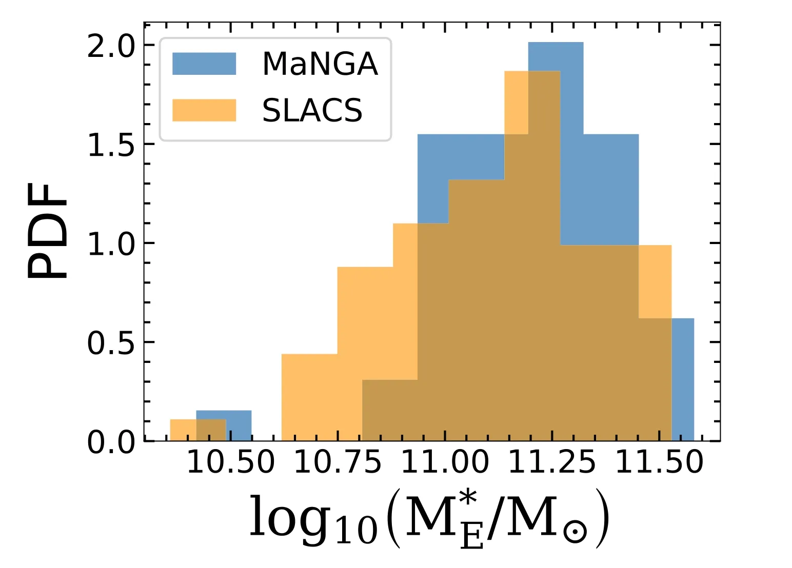
Figure A1.The PDF of the projected stellar mass within the Einstein radius of the lens galaxy,for both real SLACS lenses(orange)and our mock MaNGA lenses(blue).

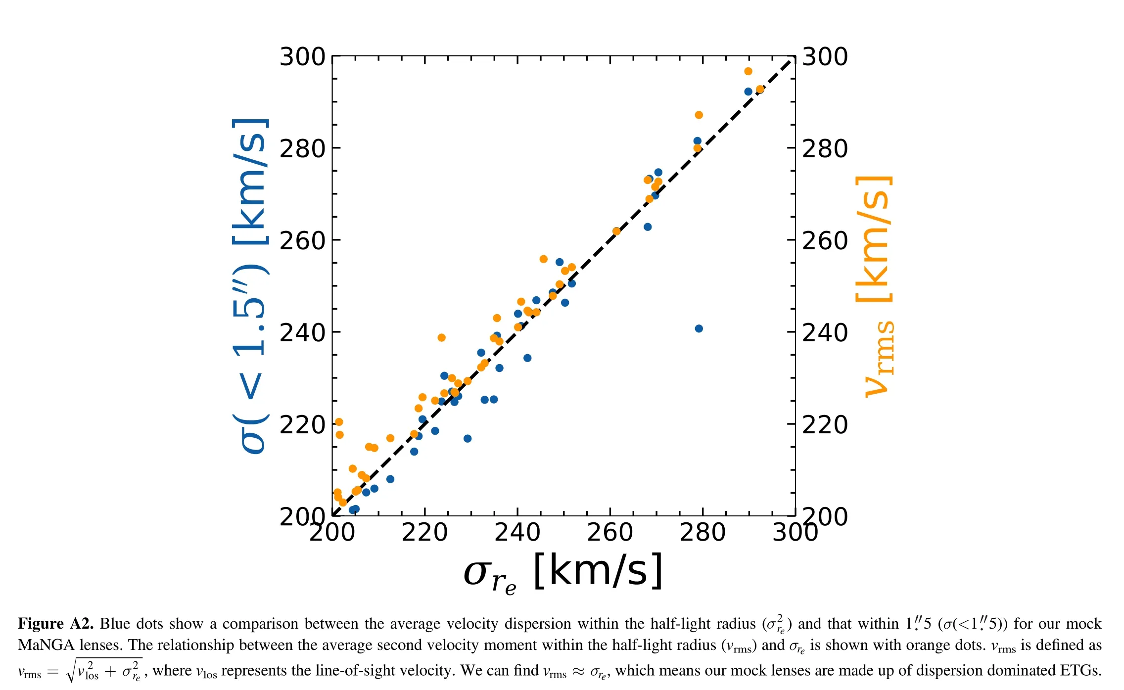
wherevlosrepresents the line-of-sight velocity.We can f indvrms≈σre,which means our mock lenses are made up of dispersion dominated ETGs.

Appendix B De flection Angle and Lensing Potential Calculation

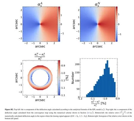
In this work,we calculate the de flection angle map numerically from the convergence map.Van de Vyvere et al.(2020)show that the truncation of the convergence map changes the symmetry of the lens’density distribution at the boundary,which may result in“pseudo shear”.To avoid this boundary effect,we need to expand the size of the convergence map when we calculate the de flection angle numerically.In Figure B1,we use an ideal EPL lens(slope=2.1,axisratio=0.6)to demonstrate this effect.The black line in the left panel is the critical line drawn based on the de flection angle given by the analytical formula of the EPL model,while the red dashed line is the critical line drawn based on the de flection angle field that is calculated numerically(with convergence map size 5″×5″).It is clear the red dashed line does not coincide with the black line,which proves that the truncation of the convergence map brings signi ficant“pseudo shear”;The right panel is the calculation result when the convergence map size is 40″×40″(the scheme described in Section 2.4).We find that the red line coincides with the black line,therefore the boundary effect can be ignored for this case.In Figures B2 and B3,we use an ideal EPL mass model to test the numerical error of the de flection angle and lensing potential calculated from the convergence.The parameter values of the EPL model are set to the typical values of our simulated lens samples(slope=2.1,Einstein radius=1 5,axis-ratio=0.8).We find that the numerical scheme described in Section 2.4 produces a numerical error of～1%for the de flection angle and lensing potential in the annular region where the lensing signal appears.Since our mock lensing images are generated from the numerically calculated de flection angles,the numerical errors we present here mean the lens galaxies in our mock data actually approach slightly biased real MaNGA ETGs.Using a higher level of oversampling(criterion-1 in Section 2.4),and increasing the size of the convergence map(criterion-2 in Section 2.4)can further reduce the numerical error of the de flection angle and lensing potential calculation.However,this requires more computational resources(currently,it takes～20 hr to calculate the convergence,de flection angle and lensing potential for each lens).The faster algorithm proposed in Shajib(2019)may be utilized in the future to overcome the numerical calculation errors due to limited computational resources.

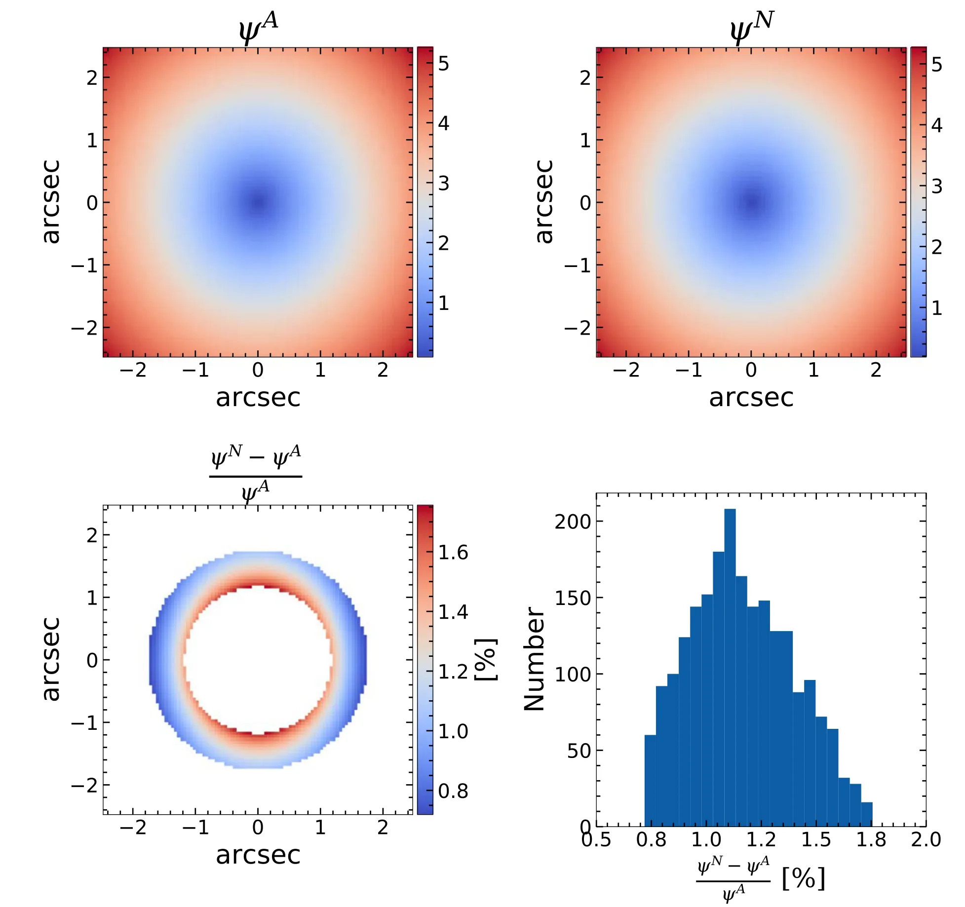
Figure B3.Similar to Figure B2,the relative error of the numerically calculated lensing potential

Appendix C Estimate the Error ofγppn

Equation(31)is equivalent to

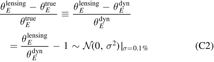
To derive the error ofγppn,we resort to the Monte Carlo way.We generate a set of discretesamples following the distribution we derived above.For each sample,we calculate the correspondingγppnvalue with Equation(C1).Eventually,the error ofγppnis given by the standard deviation value ofγppnsamples.

Appendix D Non-MST Lenses

For most outliers(9 of 11)whose physical parameters are signi ficantly misestimated,we find their existence can be understood via the MST.In this section,we present the remaining two outliers which may re flect the more complex lensing degeneracy.

Figure D1 depicts the azimuthally averaged radial pro file ofκˉ(＜θ)for lens systems“2211_8077-1902”and“559_8133-12703”.It is clearly shown that the red line,green line and orange line do not coincide so that the MST explanation discussed in Section 4.1.3 is not applicable.We further compare the de flector’s mass distribution predicted by the lens model(EPL+shear mass assumption)with that of ground truth value,and we find the difference between those two mass distributions(bottom-right panel in Figures D2 and D3)have signi ficant angular structure particularly in the region where the extended arc appears.Therefore,a uniform mass sheet is not suf ficient to compensate for the mass distribution mismatch between the ideal EPL+shear model and our mock lenses.The degeneracy in these two lens systems manifests the general Source-Position Transformation.

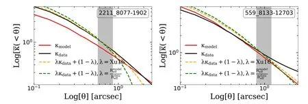
Figure D1.Similar to Figure 8,averaged radial pro file ofκˉ(＜θ)for lens system“2211_8077-1902”(left)and“559_8133-12703”(right).

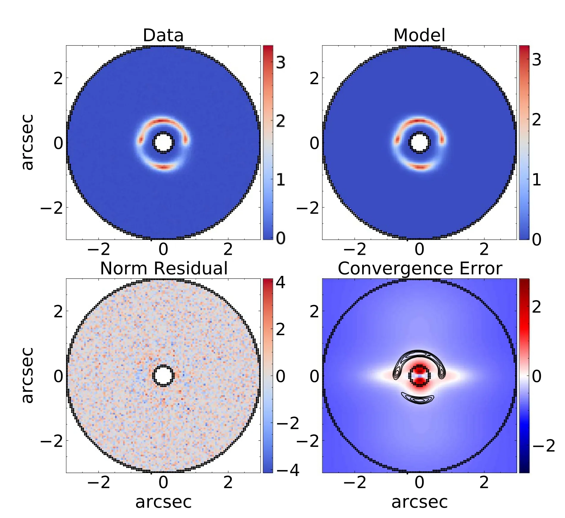
Figure D2.Similar to Figure 10,the best-fit image of the lens system“2211_8077-1902”.We can see from the bottom-right panel that the relative error map is not elliptical-symmetric,which indicates a signi ficant angular mismatch between the model and data exists.

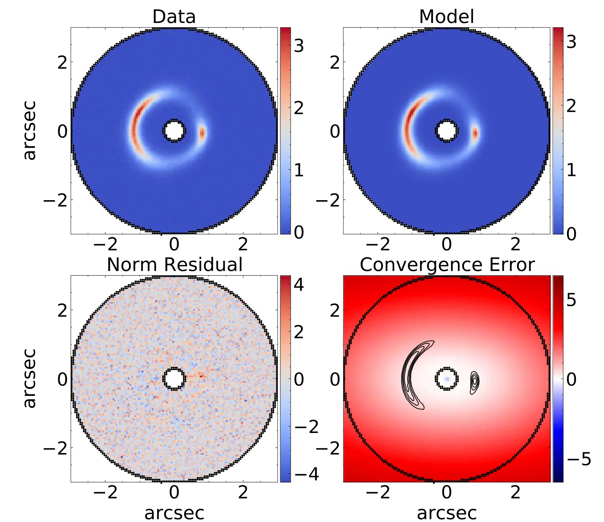
Figure D3.Similar to Figure D2,the best-fit image of the lens system“559_8133-12703”.

Appendix E H0from the Relative Time Delay

The relative time delay de fined in Equation(8)can be abbreviated as

whereηis a factor only depending on the lens and source redshift,the position of images A and B,and corresponding lensing potential values.

For our mock“MaNGA lenses”,suppose the true relative time delay between an image pair is given as

Since our image-based lens modeling cannot perfectly reconstruct the lensing potential at the location of the image pair,ηMis a biased estimation ofηD,hence our model prediction for the relative time delayΔt Mis also biased,i.e.,

Assume the time-domain observation can perfectly measure the true relative time delay(Δt D),then we can useΔt Dand the lensing potential measured from the lens model(ηM)to inferH0,

We insert Equations(E3)into(E4)to arrive at

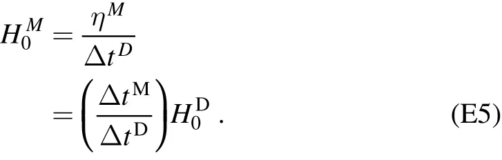
Therefore,our biased measurement of the relative time delay can be directly interpreted as a biased measurement ofH0via Equation(E5).

ORCID iDs

Xiaoyue Cao https://orcid.org/0000-0003-4988-9296