
NUMERICAL STUDY OF CAVITATION ON THE SURFACE OF THE GUIDE VANE IN THREE GORGES HYDROPOWER UNIT*
2010-05-06 08:22:26PENGYuchengCHENXiyang
水動力學研究與進展 B輯 2010年5期
PENG Yu-cheng, CHEN Xi-yang
School of energy and Power Engineering, Huazhong University of Science and Technology, Wuhan 430074, China, E-mail: fluidstar@smail.hust.edu.cn
CAO Yan
College of Electronic Information Engineering, Wuhan Polytechnic, Wuhan, 430074, China
HOU Guo-xiang
School of Traffic Science and Engineering, Huazhong University of Science and Technology, Wuhan 430074, China
NUMERICAL STUDY OF CAVITATION ON THE SURFACE OF THE GUIDE VANE IN THREE GORGES HYDROPOWER UNIT*
PENG Yu-cheng, CHEN Xi-yang
School of energy and Power Engineering, Huazhong University of Science and Technology, Wuhan 430074, China, E-mail: fluidstar@smail.hust.edu.cn
CAO Yan
College of Electronic Information Engineering, Wuhan Polytechnic, Wuhan, 430074, China
HOU Guo-xiang
School of Traffic Science and Engineering, Huazhong University of Science and Technology, Wuhan 430074, China
(Received March 7, 2010, Revised August 30, 2010)
Large-area erosions such as rust and obvious cavitation were found on the surface of the guide vane in Three Gorges hydropower units. A numerical explanation of the cavitation is given in this article. At first, based on the characteristic performance curves of the prototype hydro-turbine supplied by ALSTOM together with the actual operating conditions, an operating point is chosen for numerical analysis using the Reynolds-Averaged Navier-Stokes (RANS) equations. The flow passages from the inlet of the spiral case to the outlet of the draft tube are included in the computational domain. The results show that the static pressure on the guide vane surface is much higher than the critical pressure of cavitation. Secondly, a tiny protrusion on the guide vane surface is considered and the problem is simplified to a 2-D problem to study the local detailed flow near the guide vane surface. The protrusion is 0.5 mm in height and is 5.0 mm in width. On the basis of the results of RANS simulations, the 2-D problem is studied using the Large Eddy Simulation (LES). It is shown that there exists a region in which the static pressure reaches a level below the vapor pressure of the water. Thirdly, a cavitation model is included for the 0.5 mm protrusion case and another tiny pit case, with a tiny pit 0.3 mm in depth and 1.0 mm in width. The results show that vapor bubble exists at the protrusion entrance and the pit exit as the low pressure regions.
cavitation, guide vane, numerical analysis
1. Introduction
Static pressure governs the process of vapor bubble formation or boiling. In most cases, cavitation can occur near the fast moving blades of the turbine where the local dynamic head increases due to the action of blades which reduces the static pressure. Cavitation also occurs at the exit of the turbine when the water loses the major part of its pressure heads and any increase in dynamic head will lead to a decrease of static pressure and in its turn to cavitation.
Cavitation seldom occurs on the guide vane surface. However, large-area erosions, including roughened spots, rust and obvious cavitation erosions, were found on the suction surface of the guide vane in the Three Gorges hydropower units. The erosions of rust, damaged coating and bluing can be seen in Figs.1(a), 1(b) and 1(c), respectively. The bluing shown in Fig.1(c) is at the cavitation erosion tails.
Model tests are generally used to detect cavitation in a hydraulic turbine[1,2]and to investigate the cavitation structures[3,4]. On the other hand, the CFD is also widely and successfully used in cavitationstudies, and as a useful tool, can give realistic results in cavitation simulations[5-7]and predictions[8-10].
The article presents a study of the cavitation occurred on the guide vane surface by using numerical methods with STAR-CD commercial code. The study is divided into two steps. The first step is a steady-state RANS simulation with complete flow passages from the inlet of the spiral case to the outlet of the draft tube, to obtain the contour of the static pressure and the velocity magnitude and to verify the possibility of cavitation on a smooth guide vane surface. In the second step, a transient LES method is used for a tiny protrusion and a tiny pit on the guide vane surface, to simulate the detailed flow near the guide vane surface and to investigate the difference between the scraggly and the smooth guide vane surfaces.

Fig.1 Erosions on guide vane surface
2. Numerical analysis based on RANS equations
2.1 Geometry and discretization
The full 3-D geometry of the Three Gorges ALSTOM hydro-unit shown in Fig.2 from the spiral case to the draft tube is included for the numerical analysis to obtain the pressure distribution near the guide vane. The up right corner is the runner’s geometry, of 10.5 m in diameter.
The flow passage from the inlet of the spiral case to the outlet of the draft tube is the computational domain, which is discretized by a multi-block structured mesh. Figure 3 displays the mesh for the spiral case. Figure 4 displays the mesh for the stay vane, the guide vane and the runner. The number of stay vane blades and guide vane blades is 24. Five different hydrofoils are included in the stay vane. The number of runner blades is 15. The guide opening in Fig.2 and Fig.4 is 86%. Mesh for the draft tube is displayed in Fig.5. The total number of all meshes is 1 850 760. However, the mesh in Fig.3 to Fig.5 is the initial one, which will be adaptively refined according to yplus values.
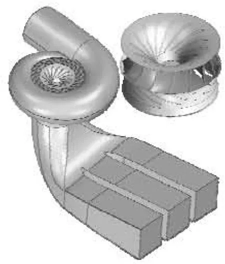
Fig.2 Full 3-D geometry and runner’s geometry (up right corner)
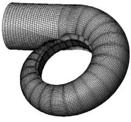
Fig.3 Mesh for spiral case
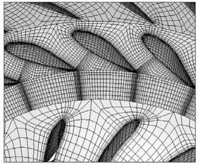
Fig.4 Mesh for stay vane, guide vane and runner
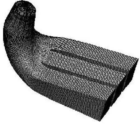
Fig.5 Mesh for draft tube
2.2 Operating condition and boundary conditions
The operating condition listed in Table 1 is chosen for the RANS simulation, which is based on the actual operating conditions and the performance curves of the prototype turbine supplied by ALSTOM Company.

Table 1 operating condition for RANS simulation
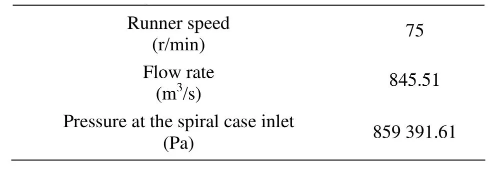
Table 2 Boundary conditions
Given the head loss in the penstock, together with the formula as shown below and Bernoulli equation, the flow rate and the pressure at the inlet of the spiral case can be obtained, which are listed in Table 2, together with the runner speed. The efficiency is expressed as
where η denotes the efficiency, P the output
Fig.6 Refined mesh near guide vane surface
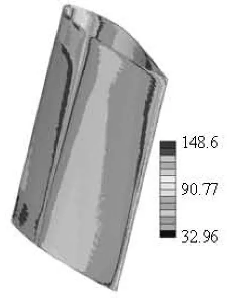
Fig.7 y+distribution on a guide vane surface
According to the formula in Ref.[12], the performance at the operating condition listed in Table 1 can be calculated as shown in the following Table 3.In addition, some other values can be obtained, for example, the thrust force acting on the runner along the axis is 12 959.81 kN, and the radial force is 208.84 kN.
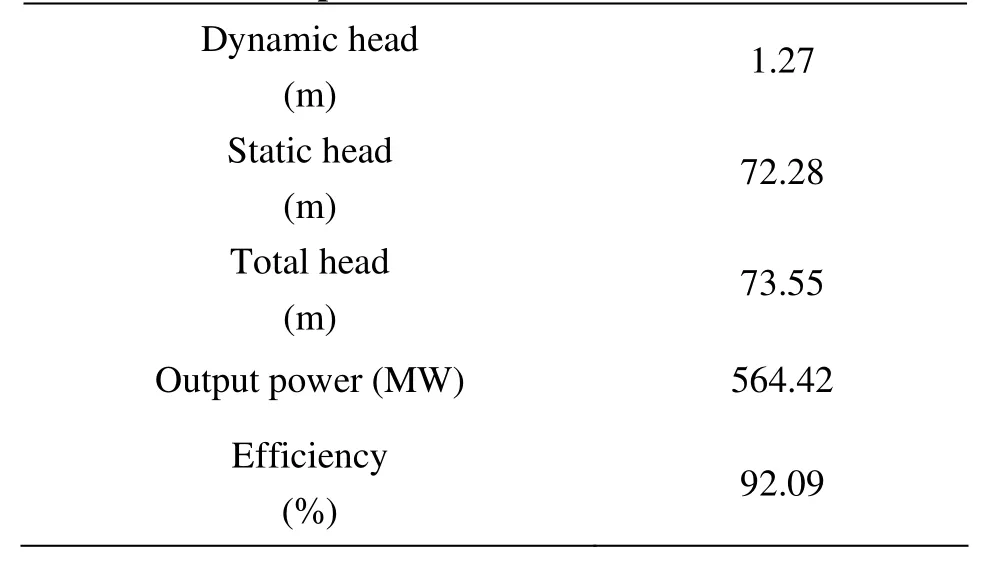
Table 3 Simulated performance
It is shown that the simulated results in Table 3 are much closer to those in Table 1.
2.4 Pressure distribution
The static pressure contour on the guide vane surface is displayed in Fig.8, where the lowest pressure on the guide vane lower exit surface is about 4.3 atmospheres, as is far above the vaporization pressure 2 370 Pa.
The lowest pressure in the full computational domain is to be found at the exit edge and the suction side of the runner blade. The lowest pressure is lower than 2 370 Pa, so cavitation may occur. Iso-surface of 2 370 Pa in the computational domain is displayed as a black area in Fig.9.
As described above, it is impossible to have conventional cavitation on a smooth guide vane, unless the pressure in all runner passages is lower than the vapor pressure of water. However, if there are some tiny protrusions or tiny pits on the guide vane surface, it will be another story. The following section will discuss the detailed flow on the guide vane surface, where a tiny protrusion and a tiny pit is considered using the LES method and the cavitation model.
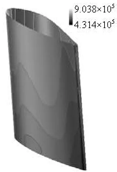
Fig.8 Pressure contour on guide vane surface
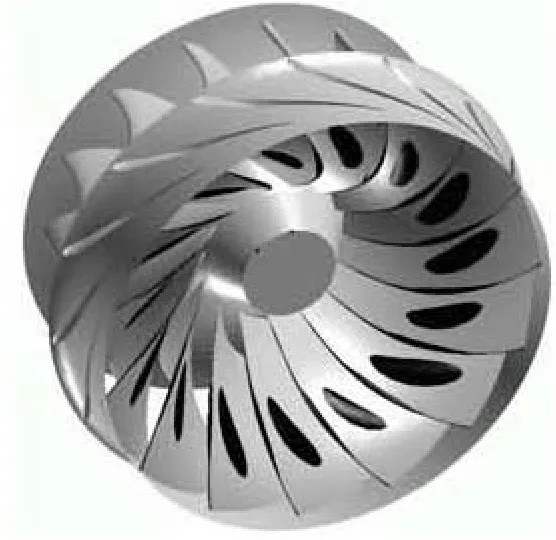
Fig.9 Iso-surface of 2 370 Pa near runner blade
3. Transient analysis based on LES
A LES in short, is a computation in which the large eddies are computed and the smallest subgrid-scale (SGS) eddies are modeled. Literature[13]conducted a numerical modeling study using the 2-D LES approach to evaluate the wind effects on the transport and dispersion processes close to a covered roadway. The LES results, although only two dimensional, are in a good quantitative agreement with the experimental data and only slightly overestimate the concentration levels. The covered roadway is similar with the geometry used in our article. Therefore the 2-D LES will be used in our study. Further investigations will be conducted in order to compare the results of 2-D and 3-D computations.
3.1 Geometry and boundaries
A tiny protrusion is considered on the guide vane surface in this section. The geometry is simplified to a 2-D problem as shown in Fig.10, together with the primary direction of flow.
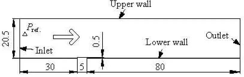
Fig.10 Geometry and boundaries (mm)
At the entrance of the geometry, the velocity inlet boundary is specified. At the exit is the outlet boundary. At the lower wall, the standard wall function is used. In addition, at the upper wall, the frictionless slip wall is assumed to avoid its influence. The location of the reference pressure, Pref, is marked in Fig.10.
Structured mesh is used and the meshes near theprotrusion are refined as shown in Fig. 11. The total number of finite volume cells is 86 580.
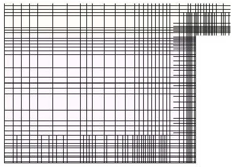
Fig.11 Meshes near protrusion
The velocity at the entrance and the reference pressure are chosen according to the RANS results. The velocity magnitude distribution and the pressure distribution at the mid section plane of the guide vane is shown in Fig.12 and Fig.13, respectively. It can be seen that the velocity at the inlet boundary is 21 m/s, and the pressure at the reference location (see Fig.10) is 6.4×10⁵Pa.
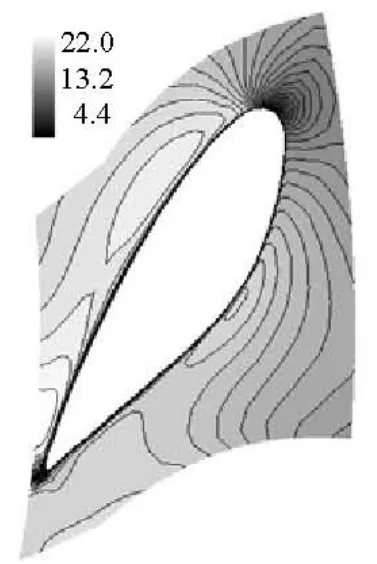
Fig.12 Velocity magnitude distribution at the mid section plane of the guide vane
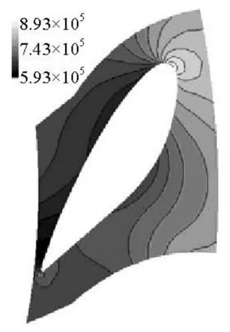
Fig.13 Pressure distribution at the mid section plane of the guide vane
3.2 Results without using the cavitation model
The Smagorinsky mode[14]is used to solve this problem. To obtain the best results from LES, second-order schemes are used for both the temporal and spatial discretization, with time step of 1×10⁻⁶s.
Figure 14 shows the contour plot of the instantaneous static pressure. The deep color denotes the low pressure. The region in which the static pressure reaches a level below the vapor pressure of the water can be distinguished.
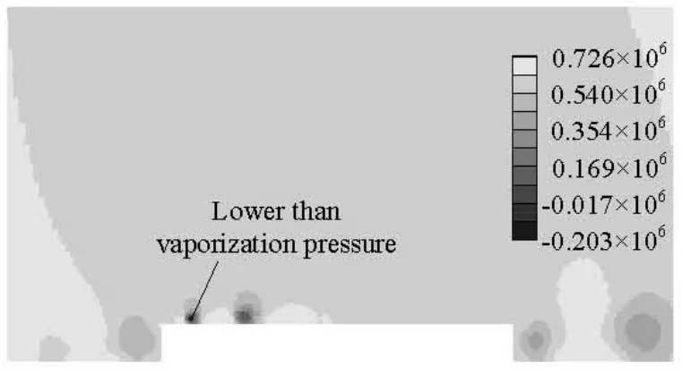
Fig.14 Contour plot of the instantaneous static pressure without using the cavitation model
3.3 Results obtained by using the cavitation model
In this case, the barotropic model[15]is used to simulate cavitation. The result is displayed in Fig.15. Deep color means a low pressure. It is shown that there is a vapor bubble at the entrance of the protrusion.
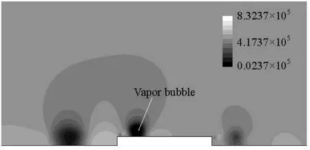
Fig.15 Contour plot of pressure obtained by using the cavitation model
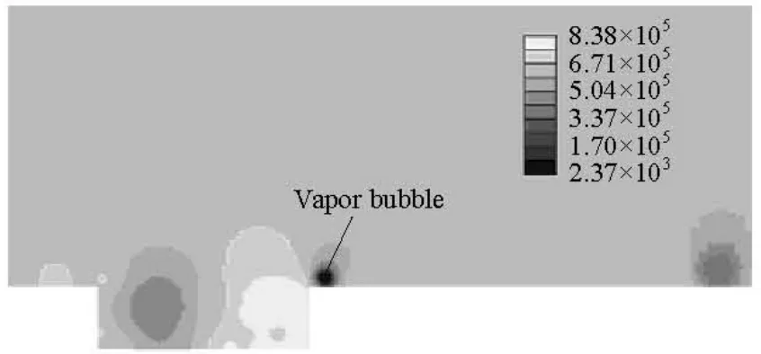
Fig.16 Contour plot of pressure
3.4 Another case
In this case, a 2-D tiny pit of 1 mm in width and 0.3 mm in depth is considered. Other geometry and boundary conditions are the same as those in Fig.10. The pressure contour at an instant is obtained by usingLES and the cavitation model is shown in Fig.16. Deep color means a low pressure in this figure. It is shown that there exists a vapor bubble at the exit of the pit.
4. Conclusions
The RANS equations are solved in the computational domain comprising the flow passages from the inlet of the spiral case to the outlet of the draft tube. An operation condition is chosen for the simulation based on the actual operation conditions and the characteristic performance curves of prototype hydro turbine supplied by ALSTOM. It is found that the simulated performance agrees well with the actual one. Meanwhile, the contour of the static pressure on the guide vane surface indicates that it is impossible to have conventional cavitation on a smooth guide vane.
However, if there are tiny protrusions or tiny pits on the guide vane surface, it will be another story. Considering a tiny protrusion of 5 mm in width and 0.5 mm in height and a tiny pit of 1.0 mm in width and 0.3 mm in depth on the guide vane surface, the detailed flow near the protrusion and the pit is computed using the LES method. The boundary conditions are determined by the pressure contour and the velocity magnitude contour at the mid section of the guide vane obtained from the RANS simulation. The LES results show that there is a region in which the absolute static pressure is under the vapor pressure of the water. Further simulations by using the cavitation model show that there are vapor bubbles in the flow domain. Therefore, it can be said that the cavitation will occur only if the guide vane surface is scraggly, such as with deciduous coat or tiny pits caused by silt cutting.
[1] ESCALER X., EGUSQUIZA E. and FARHAT M. et al. Detection of cavitation in hydraulic turbines[J]. Mechanical Systems and Signal Processing, 2006, 20(4): 983-1007.
[2] MASJEDIAN JAZI A., RAHIMZADEH H. Detecting cavitation in globe valves by two methods: Characteristic diagrams and acoustic analysis[J]. Applied Acoustics, 2009, 70(11-12): 1440-1445.
[3] METTIN R., LUTHER S. and OHL C. D. et al. Acoustic cavitation structures and simulations by a particle model[J]. Ultrasonics Sonochemistry, 1999, 6(1-2): 25-29.
[4] DULAR M., BACHERT B. and STOFFEL B. et al. Relationship between cavitation structures and cavitation damage[J]. Wear, 2004, 257(11): 1176-1184.
[5] LIU De-min, LIU Shu-hong and WU Yu-lin et al. LES numerical simulation of cavitation Bubble shedding on ALE 25 and ALE 15 hydrofoils[J]. Journal of Hydrodynamics, 2009, 21(6): 807-813.
[6] WANG G., OSTOJA-STARZEWSKI M. Large eddy simulation of a sheet/cloud cavitation on a NACA0015 hydrofoil[J]. Applied Mathematical Modelling, 2007, 31(3): 417-447.
[7] POUFFARY B., PATELLA R. F. and REBOUD J. L. et al. Numerical simulation of 3D cavitating flows: Analysis of cavitation head drop in turbomachinery[J]. Journal of Fluids Engineering, 2008, 130: 061301.
[8] PARK K., SEOL H. and CHOI W. et al. Numerical prediction of tip vortex cavitation behavior and noise considering nuclei size and distribution[J]. Applied Acoustics, 2009, 70(5): 674-680.
[9] HATTORI S., KISHIMOTO M. Prediction of cavitation erosion on stainless steel components in centrifugal pumps[J]. Wear, 2008, 265(11-12): 1870-1874.
[10] YE Jin-ming, XIONG Ying. Prediction of podded propeller cavitation using an unsteady surface panel method[J]. Journal of Hydrodynamics, 2008, 20(6): 790-796.
[11] MENTER F. R. Zonal two equation k-ω turbulence models for aerodynamic flows[C]. Proc. 24th Fluid Dynamics Conference. Orlando, Florida, USA, 1993, AIAA 93-2906.
[12] PENG Yu-cheng. Research on the abnormal vibration of unit 6 of the Three Gorges Left Bank Station under small guide opening conditions[D]. Ph. D. Thesis, Wuhan: Huazhong University of Science and Technology, 2007(in Chinese).
[13] LAATAR A. H., BENAHMED M. and BELGHITH A. et al. 2D large eddy simulation of pollutant dispersion around a covered roadway[J]. Journal of Wind Engineering and Industrial Aerodynamics, 2002, 90: 617-637.
[14] SMAGORINSKY J. General circulation experiments with the primitive equations, Part I: The basic experiment[J]. Mon. Weather Rev., 1963, 91(3): 99-115.
[15] SCHMIDT D. P., RUTLAND C. J. and CORRADINI M. L. A numerical study of cavitating flow through various nozzle shapes[J]. SAE Trans., 1997, 106(3):1664-1673.
10.1016/S1001-6058(09)60106-2
* Project supported by the National Natural Science Foundation of China (Grant Nos. 50975103 and 51006039).
Biography: PENG Yu-cheng (1975-), Male, Ph. D., Lecturer
HOU Guo-xiang, E-mail: houguoxiang@163.com

- 水動力學研究與進展 B輯的其它文章
- NUMERICAL SIMULATION OF THE ENERGY DISSIPATION CHARACTERISTICS IN STILLING BASIN OF MULTI-HORIZONTAL SUBMERGED JETS*
- ANALYSIS OF EDL EFFECTS ON THE FLOW AND FLOW STABILITY IN MICROCHANNELS*
- EXPERIMENTAL INVESTIGATION ON THE DRAG REDUCTION CHARACTERISTICS OF TRAVELING WAVY WALL AT HIGH REYNOLDS NUMBER IN WIND TUNNEL*
- NUMERICAL MODELING PURIFICATION PERFORMANCE OF POT TEST*
- A NEW METHOD FOR NUMERICAL SIMULATION OF TWO TRAINS PASSING BY EACH OTHER AT THE SAME SPEED*
- THE COMPARATIVE STUDY OF VENTILATED SUPER CAVITY SHAPE IN WATER TUNNEL AND INFINITE FLOW FIELD*