Xi-zeng Zhao, Tian-yu Xu, Zhou-teng Ye, Wei-jie Liu

1. Ocean College, Zhejiang University, Zhoushan 316021, China

2. The Engineering Research Center of Oceanic Sensing Technology and Equipment, Ministry of Education,Zhejiang University, Zhoushan 316021, China

Abstract: In this study, a computational framework in the field of artificial intelligence was applied in computational fluid dynamics(CFD) field. This Framework, which was initially proposed by Google AI department, is called “TensorFlow”. An improved CFD model based on this framework was developed with a high-order difference method, which is a constrained interpolation profile (CIP)scheme for the base flow solver of the advection term in the Navier-Stokes equations, and preconditioned conjugate gradient (PCG)method was implemented in the model to solve the Poisson equation. Some new features including the convolution, vectorization, and graphics processing unit (GPU) acceleration were implemented to raise the computational efficiency. The model was tested with several benchmark cases and shows good performance. Compared with our former CIP-based model, the present TensorFlow-based model also shows significantly higher computational efficiency in large-scale computation. The results indicate TensorFlow could be a promising framework for CFD models due to its ability in the computational acceleration and convenience for programming.

Key words: TensorFlow, vectorization, Navier-Stokes equations, graphics processing unit (GPU) acceleration, constrained interpolation profile (CIP) method, preconditioned conjugate gradient (PCG) method

Introduction

Computational fluid dynamics (CFD) models directly solving Navier-Stokes (N-S) equations are convenient tools to study problems involving water flows. It is well known that the computational efficiency is the main limitation of a CFD model when it comes to complex physical problems . Therefore,researchers have devoted their efforts to accelerating the computation of CFD models. Among various computational acceleration methods, graphics processing unit (GPU) acceleration is one of the useful methods. Despite the rapid development of central processing units (CPUs), GPUs usually have the advantage of higher computational efficiency especially when the grid number is very large. A number of researchers have successfully applied GPU acceleration for CFD model calculations[1-2]. However,in order to take advantage of GPUs, researchers are supposed to get knowledge of how to program based on compute unified device architecture (CUDA)[3]or Open Computing Language (OpenCL)[4]while some researchers may not be familiar with CUDA or OpenCL frameworks. This might hinder the wide application of GPU acceleration in the CFD field. In this paper, a new framework called TensorFlow is introduced as an optional solution to the problem mentioned above. TensorFlow is a popular opensource framework for high-performance computation,initially developed by Google AI Department[5]for computational acceleration in machine learning or deep learning. Nowadays, there are also other frameworks or open-source libraries available for the CFD field, such as OpenFOAM and Reef 3D. Many practical problems have been studied using these open-source tools, such as turbulent flow past a square cylinder[6], wave simulations[7], bubble drag reduction[8], inner flow in a pump[9], etc.. Self-defined algorithms can also be developed based on OpenFOAM[10]or Reef 3D[11]. Compared with these frameworks, TensorFlow has the following advantages. Firstly, TensorFlow is operational in all platforms including Windows, Mac OS, Linux (even Android and iOS) while OpenFOAM and Reef 3D are not recommended to be installed on the Windows system due to the numerical instability. Secondly,OpenFOAM and Reef 3D only adopt C++ as the coding language, while TensorFlow offers multiple choices including Python, C++, Java, etc.. Thirdly,TensorFlow APIs are optimized specially for large-scale computation, and also helps to realize distributed computation and GPU acceleration easily.Those researchers who know little about GPUs may also be able to apply them in the computational acceleration. Fourthly, a lot of TensorFlow application programming interfaces (APIs) have strong links to artificial intelligence, which may be extended to CFD models in future work.

Considering these advantages, a new CFD model with high-performance computational ability was developed based on the TensorFlow framework. The model works on the Cartesian grid system and finite difference methods are applied. In this model, the constrained interpolation profile (CIP) method is used to discretize the convection term of N-S equations. The CIP method, which is a third order finite difference scheme to solve the hyperbolic partial differential equations, was used to solve hyperbolic equations[12].Our former model, which is called CIP-based model,has been successfully applied in many cases such as dam break[13]and Fluid-structure interaction[14-15].Besides, the preconditioned conjugate gradient (PCG)method, which is a widely used iterative method for solving sparse matrices, is implemented in the present model to solve the Poisson equation. The Conjugate Gradient method was popularized by Reid[16]as an iterative solver for large and sparse matrices. In linear algebra, preconditioning is A universal method to obtain a more rapid convergence and the PCG method is more commonly used rather than the conjugate gradient method. Nowadays many preconditioners are available such as the Jacobi preconditioner, incomplete Cholesky factorization, sparse approximate inverse(SPAI) preconditioner, successive over-relaxation precondi- tioner, etc.. In the present work, we packaged the CIP scheme and the PCG method as optimized modules in a vectorized version, which were specially designed for the computational efficiency of our model.The present model was tested with various benchmark cases. The first case is Zalesak’s advection test selected to verify the advection solver in our TensorFlow-based model with the CIP scheme. The second case is selected to verify the Poisson equation solver with the PCG method. The other two cases of lid-driven cavity flow and flow over a circular cylinder are selected to demonstrate the accuracy and computational efficiency of the model. As a preliminary test to prove the high-performance computational ability, the free surface is not included and left for future work.

1. Mathematical method

1.1 Governing equations

The governing equations adopted in the present model are N-S equations for the incompressible viscous fluid. The continuity and momentum equations are expressed as:

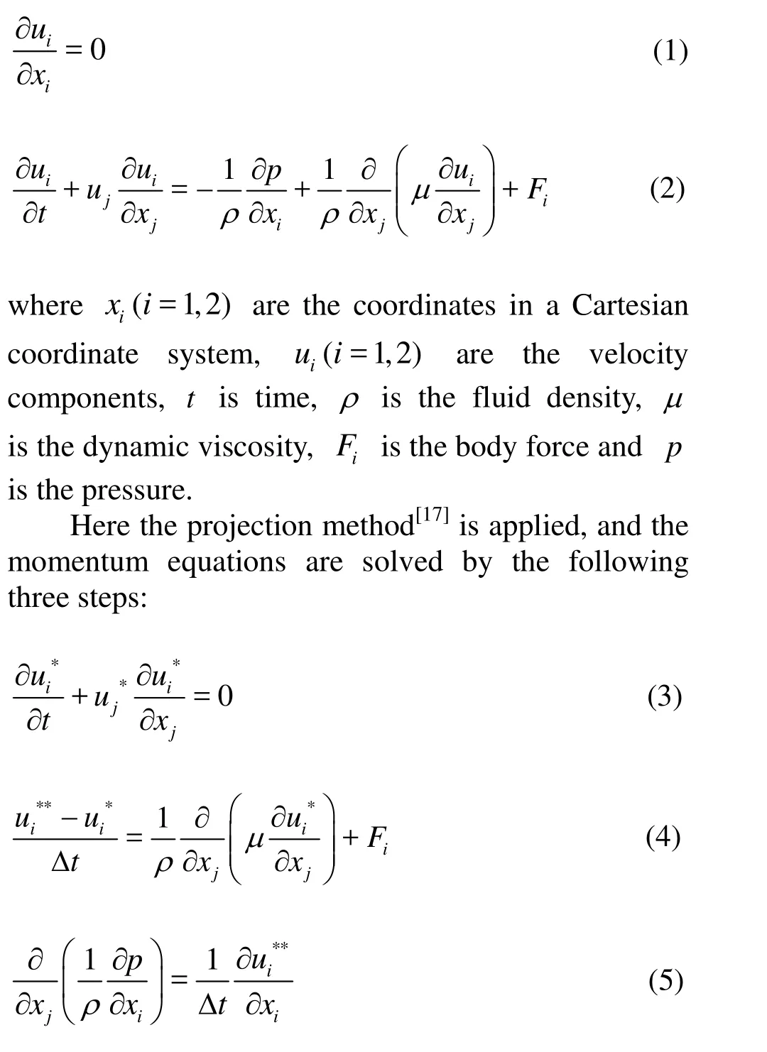
In the first step, we neglect the diffusion term and pressure term as seen in Eq. (3). The CIP method is used to solve this equation and the solution is u*,which is considered as an intermediate velocity. In the second step, a central difference scheme is used to calculate the gradient of the non-advection term of Eq.(4) and the solution is u**, which is a renewed intermediate velocity. In the third step, the pressure coupling with the velocity field is calculated using a PCG method. Then the flow field data are updated and these steps continue as a circle until the end of the simulation. The details of the flow solver can be found in previous studies[13].

1.2 Fluid and structure interactions

In order to deal with the fluid-structure interaction, an immersed boundary method[18]is applied. The velocities in the computational domain can be obtained by where u is the flow velocity of the fluid, Ubis the velocity of the solid object, φ stands for the solid phase and 1-φ stands for the liquid phase.

1.3 The CIP scheme

The main idea of the CIP scheme is that when calculating the advection Eq. (7), the transportation equation of f, as well as its spatial gradient g=?f/?x are both applied.

For simplicity, we take the 1-D advection with a constant advection velocity of u>0 as an example.Figure 1(a) shows the initial profile and the exact solution after advection at discretized points as shown in Fig. 1(b). In the CIP scheme, we approximate a profile for fninside the upwind cell [xi-1,xi] as:

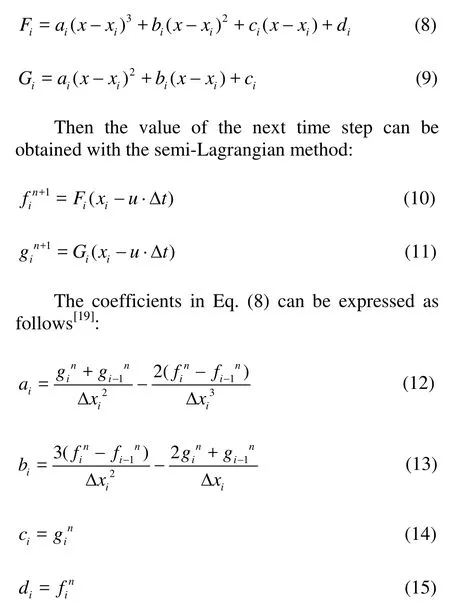
Figures 1(c) and 1(d) shows the corresponding solutions from the linear interpolation scheme and CIP scheme respectively.

1.4 The preconditioned conjugate gradient method

Theconjugategradientmethod[20]isusedin machine learning and deep learning to solve the linear system of equations with sparse matrices and it’s also applicable in the CFD field. It has the advantages of fast convergence and high calculation stability.Moreover, the precondition is usually used to increase the convergence speed.

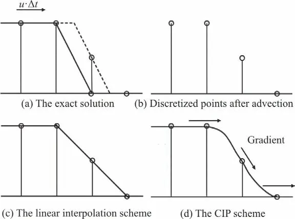
Fig. 1 The introduction of CIP method

The linear equations system can be written as Ax = b . When using the preconditioned conjugate gradient (PCG) method to solve this linear equations system, A should be a symmetrical positive determined matrix with the size of N × N , where N is a positive integer. Assuming the exact solution of x being 0 x , we define the error as 0 = i i e x - x , and define the residual as = i i r b - Ax (where i x stands for the numerical result solved in an iterative way, and i is the number of iterations), which both have the size of N ×1. The iteration step goes as:

where βi+1=(ri+1Tri+1)/riTri. βiis the step length of each iteration. After certain finite iterations, an approximate numerical solution can be obtained. As the iteration step increases, the residual can be reduced as small as possible. A precondition is usually implemented to achieve a high convergence speed.The precondition is a technique which can improve the condition number of a matrix and make it easier to be solved. In our TensorFlow-based model, one of the widely used pre-conditioners, which is called Jacobi pre-conditioner, is chosen to solve the Poisson equation because of its simplicity and time-saving characteristics in the calculation.

1.5 Convolution and vectorization tricks

Different from our former CIP-based model,convolution and vectorization are applied in the present model to accelerate the calculation.

The idea of using convolution kernels to capture flow field features is inspired by the convolutional neural networks (CNN), which is specially designed for computer vision and image processing. As image pixels are similar to grids, convolution can also be applied in CFD models. It should be pointed out that convolution is one of the built-in functions in TensorFlow, which not only can be directly used but also specially optimized for large-scale computation.Figure 2 is shown to illustrate how it works.

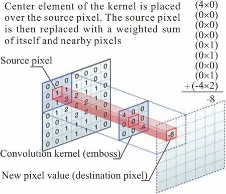
Fig. 2 (Color online) Convolution process

As illustrated in Fig. 2, we avoid the loop but make a convolution kernel to realize the finite difference scheme in TensorFlow.

For example, when calculating Δf/Δx=(fi+1,j-fi-1,j)/(xi+1,j-xi-1,j), the designed convolution kernel and the corresponding value of f are shown in Fig. 3.

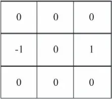
Fig. 3(a) Convolution kernel

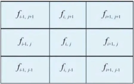
Fig. 3(b) (Color online) The corresponding value of f

The numbers of 0, -1 and 1 in this convolution kernel stand for weight coefficients, which will multiply the corresponding value of f and the weighted sum will be calculated as the result after this convolution process. The same convolution kernel will be applied to the numerator and denominator respectively, which means:

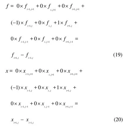
In this way, the finite difference scheme in the model can be realized with different convolution kernels.And it should be pointed out that after the convolution process, the boundary values are supposed to be corrected according to the boundary conditions.

Vectorization is the process of reconstructing a loop using certain instruction sets such as single instruction multiple data (SIMD) or multiple instruction multiple data (MIMD). Instead of processing individual elements in an array or matrix for multiple times, vectorization will process them entirely.

Here is the example code to illustrate the differences between the traditional form and the vectorization form. A and B are both data arrays with the same type of 1×N, where N is an integer.

The traditional form

The vectorization form

In this way, the computational resources can be fully used and thus a lot of computational time can be saved. Generally speaking, vectorization may accelerate several times compared with using loops in the calculation. As a result, most loops have been replaced by vectorization in the present TensorFlowbased model, in which case the computational efficiency is greatly improved.

1.6 Implementation of the CFD solver

The details of solving a CFD problem in TensorFlow are introduced in this section.TensorFlow executes the calculation in the form of computation graphs (Fig. 4), with every single node standing for a calculation operation, and each operation may obtain zero or several inputs and outputs. All nodes are designed previously in operation libraries using the advanced language,Python. The simulation runs in the form of a session,which is executed in C++ to increase computational speed. Besides, TensorFlow has its own computational logic system and unique way to process data.All data is calculated and stored as a special data type called “tensor”, which is specially optimized for the large-scale computation.

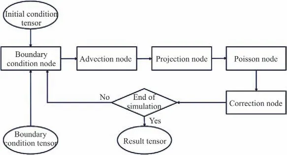
Fig. 4 The computation graph

As seen in Fig. 4, at the very beginning, initial conditions, boundary conditions, and convolution kernels are supposed to be specified. Assuming that the current time step is n, and the velocity and pressure can be marked as unand pnrespectively.Then the advection term of Eq. (3) is firstly solved and the intermediate velocity u*is obtained. After projection operation, a renewed intermediate velocity of u**in Eq. (5) is obtained. Due to the fact that the pressure and velocities are highly coupled, in the Poisson Node, the pressure of the next time step,which is marked asn+1p is solved in an iterative way using the PCG method. At last in the Correction Node,the velocity ofn+1u is rectified. In this way, the loop of updating the velocities and pressure is completed.In addition, if the current time step is not the end step,the loop will continue to be executed, otherwise, the total simulation will come to the end.

Details of the CIP module and the PCG module are explained in this paragraph. The CIP module consists of two parts: the first part works for calculating the necessary coefficients of the CIP solver (e.g., for 2-D cases, totally 7 coefficients marked as A1-A7), and the second part works for calculating results in a vectorized way as follows:

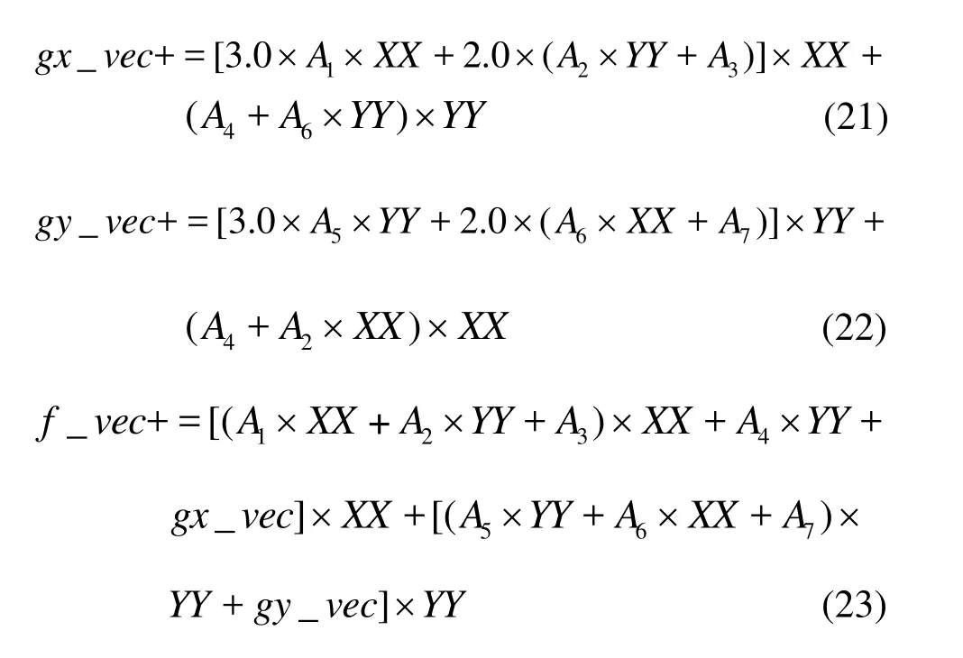
where XX=-u×dt, YY=-v×dt (u and v are velocities). The result of f_vec is what we needed,and gx_vec, gy_vec are its gradient values in x,y directions, respectively. The PCG module also consists of two parts: the first part is to apply the preconditioner, and the second part is to solve the matrix with CG. In the second part, two factors including the step length, step direction are supposed to be specified. The iteration goes in the following way: x_vec+=alpha×r, where alpha is the step length, r stands for the iterative direction. This iteration also works in a vectorized way in order to optimize the computational speed.

2. Tests and validations

In this section, several tests are performed to prove the validity of our TensorFlow-based model.All tests in this paper are conducted using the same computational devices, whose GPU is NVIDIA GeForce GTX Titan Black with 6G memory and CPU is Intel (R) Core (TM) i7-6700K CPU@4.00GHz.

2.1 CIP scheme validation

To evaluate the performance of the CIP method based on the Tensorflow framework, Zalesak’s test[21]was simulated. Zalesak’s test, also called solid body rotational problem, is a classical test for advection flow. The motion of Zalesak’s solid body is governed by the advection equation

Fig. 5 (Color online) (a) The initial state of the Zalesak’s solid body (b)-(d) The result after a period of advection with the grid number being 100×100, 200×200 and 400×400. Three contour lines stand for the values of 0.05, 0.50 and 0.95, respectively

The velocities are given as follows:u=ω(y-0.64) and v =ω(0.64-y), where ω is 1.0, standing for the angular velocity. The value of f inside the cut-out circle is 1.0, and outside is 0. The computational domain is [0m,1.28m]×[0m,1.28m],and the grid space is 0.0064 m. Time step is 0.00314 s.The number of total steps is 2 000 and thus the total simulation time is 6.28 s. Figure 5 shows the results of this problem after one complete revolution, with the grid number being 100×100, 200×200 and 400×400 respectively.

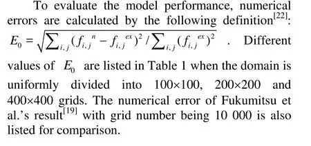
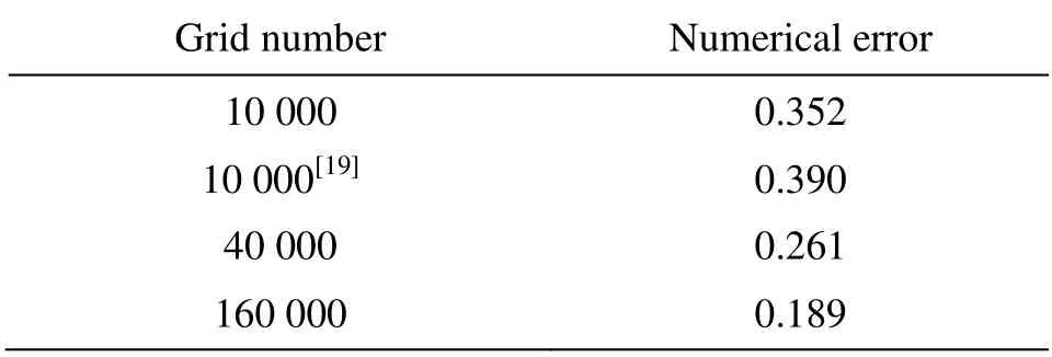
Table 1 Numerical errors of Zalesak’s test

2.2 Poisson equation solver

In this section, the performance of the Poisson equation solver in the TensorFlow-based model is tested. Equation (5) is a typical expression of the Poisson equation. As we assume no free surface in the computational field, the fluid density can be treated as a constant and therefore Eq. (5) can also be written as?2p=ρ/Δt(?u/?x+?v/?y). In this equation, the velocities and pressure are fully coupled, which means pressure can be obtained from velocities through iterations. In other words, we are solving a linear equation system Ax=b iteratively, where A is the coefficient matrix, x is pressure (p) in the Poisson equation above and b is the term on the right side,which is equal to ρ/Δt(?u/?x+?v/?y) solved in a numerical way.

The velocities are given as:

Preconditioned conjugate gradient method is applied to solve the linear equation system and Jacobi pre-conditioner is taken as the default pre-conditioner.Here the residual, which can be expressed as?2p-ρ/Δt(?u/?x+?v/?y), is defined as the difference between the numerical and analytical solution. The total residual of the Poisson equation is defined as L2 Norm(r)=∑ri,j2, where ri,jis the residual of each grid point. The computation domain is [0m,2m]×[0m,2m], divided into 500×500 grids.The value of fluid density is assumed as 1.0 kg/m3and the time step is set to 0.01 s. We defined a parameter named “tolerance”, the value of which can be given by users to adjust the convergence precision. The results of the Poisson equation with different tolerances are listed in Table 2, which shows that the PCG Poisson solver used in the present model is quite reliable. Figure 6 shows the numerical solution of pressure, which is noted as p in Eq. (5). Figure 7(a)is the analytical solution of ?2p and Fig. 7(b) is the numerical solution of ?2p, in which case the tolerance is set as 10-4. Qualitatively, they show good agreement. Figure 8 illustrates residuals of the Poisson equation when different tolerance values are given for quantitative comparison. The results show that our Poisson solver is highly precise and is workable for our model.

Table 2 Results of the Poisson equation with different tolerances

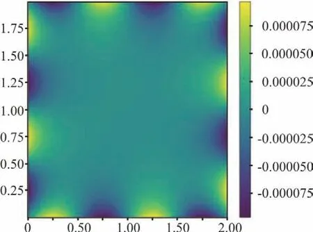
Fig. 6 (Color online) The numerical results of pressure distribution

2.3 Lid-driven cavity flow

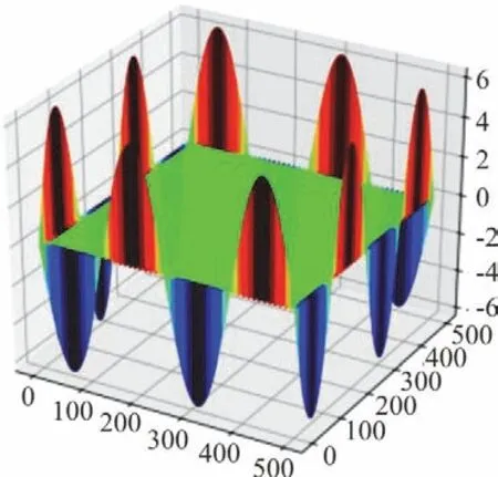
Fig. 7(a) (Color online) Analytical solution of ?2p

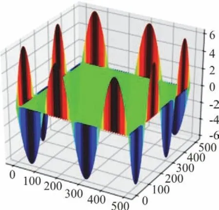
Fig. 7(b) (Color online) Numerical solution of ?2p

The lid-driven cavity flow is considered as the classical test problem for the validation of numerical methods and codes for solving N-S equations. The case was simulated to prove the validity of the solver in our TensorFlow-based model as well as its high-performance computational ability. In the simulation of this case, the total simulation time is 100 s with the time step, 0.0005 s. The computational domain is [0m,2.56m]×[0m,2.56m]with the grid number, 160×160, and no-slip boundary conditions are specified. The horizontal velocity u on the top side where y=2.56 is set to -1 m/s, and on the other three sides the values of u are 0. Besides, the vertical velocity v is 0 on each side of the boundaries. The fluid density is 1.0 kg/m3, and the Reynolds number is 1000. It has been verified that the solution obtained at Re=1000 is quite close from one author to another[23]. Thus, our results are compared with Ghia’s classical results[24]as well as CIP-based model’s results to prove the validity of the present model as shown in Fig. 9. The lengths of the cavity edges are marked as xm and ym in Fig. 9.

It should be pointed out that different Poisson equation solvers are implemented in the present model and CIP-based model, which call for different convergence criterions. In our TensorFlow-based model, the PCG solver is applied and the criterion is restricting residuals of the whole linear equations system, while in the CIP-based model, the SOR method is used and the criterion is restricting max differences between two consecutive iterations. Theoretically, it is hard to determine which criterion is better, while it can be seen from Fig. 9 that the TensorFlow-based model performs better with the same tolerance value assigned (tolerance=1×10-3).

Fig. 8 (Color online) Residuals of the Poisson equation with different tolerances

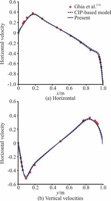
Fig. 9 (Color online) Comparisons of the results from the present model, CIP-based model and Ghia[24]

The streamline, pressure, and vortex distribution are also plotted in Fig. 10. As seen in Fig. 10(a), there are three vortices. One is the primary vortex and the other two are secondary vortices. Figures 10(b) and 10(c) show the vortex distribution and the pressure distribution respectively. Bruneau et al.’s results[23]are also displayed in Fig. 11 for comparison. It can be noticed that predicted results from the present model agree qualitatively well with their results.

Table 3 and Fig. 12 show the computational time of the TensorFlow-based model and CIP-based model with different grid numbers. When the grid number is small, the time of data transport and exchange on the GPU can not be neglected compared to the total computational time so that the efficiency of GPUs is relatively lower than CPUs. However in the large-scale computation, this cost can be negligible and as the grid number increases, the computational time of the CIP-based model increases much faster than the TensorFlow-based model. With the help of the convolution, vectorization and GPU acceleration skills, our TensorFlow-based model may work more than 10 times faster than the CIP-based model. It should be noticed that, due to different Poisson solvers and convergence criterions used in these two models,it’s very hard to produce results with the same precision and our idea is to prove that the TensorFlow-based model works not only better but also faster than the CIP-based model with the same tolerance value assigned, which is 1×10-3in this case.

Fig. 10 (Color online) The streamlines, vortex, and pressure distribution of the lid-driven cavity flow test’s steady solution at Re=1000

2.4 Flow past a circular cylinder

Fig. 11 Bruneau et al.’s results of the lid-driven cavity flow test’s steady solution at Re=1000[23]

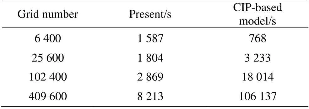
Table 3 The computational time of the TensorFlow-based model and CIP-based model with different grid numbers

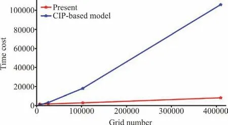
Fig. 12 (Color online)The computational time ofthe TensorFlow-based model and CIP-based model with different grid numbers

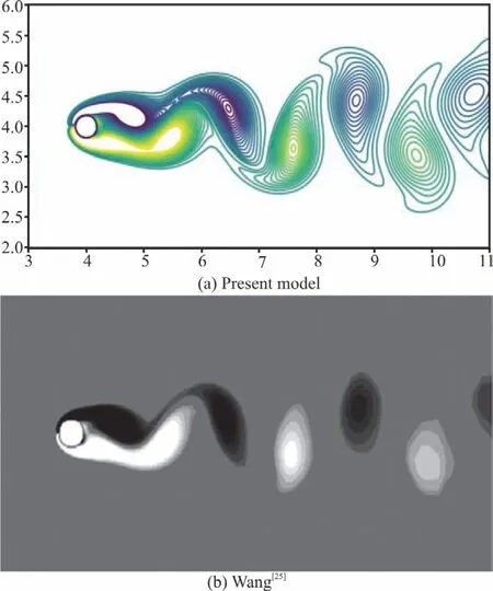
Fig. 13 (Color online) Vortex shedding simulated by the (a)present model and (b)Wang[25]

The 2-D flow past a stationary cylinder was also simulated using the immersed boundary method. This case is a test about the model performance for fluidstructure interactions as well as computational efficiency. The simulation was performed in a rectangular domain of [30D,20D], where D=0.4m is the radius of the cylinder. The circular cylinder’s center is located at x=10D, y=10D in the computational domain.The Newman boundary condition is specified on the top, bottom and outlet boundaries. The grid space is set as D/ 25 and the time step is 0.0005 s. A constant velocity of u =1m/s is given at the domain entrance. The liquid density is 1.0 kg/m3, and the Reynolds number is 100. It has been found in this case that the vortices begin shedding regularly when the simulation time is longer than 80s. Therefore the total simulation time is set as 120 s. Figure 13(a) is the vortex distribution at t =120 s . Figure 13(b) shows Wang’s results[25]with the same Reynolds number and our result shows similar locations and shapes of the shedding vortices.

In order to make a quantitative comparison, the drag and lift coefficients are generally calculated as:

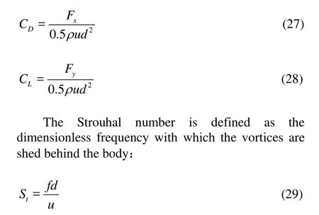
The results of the Tensorflow-based model and CIP-based model with different grid resolutions are listed in Table 4. In this case, the tolerance value is set as 1×10-4. The coarse grid space is D/20, the middle one is D/25, and the fine one is D/32. As seen in Table 4, the results of two models show good agreement. Predicted results from the Tensorflowbased model with the fine grid size and existing literature data are listed in Table 5. As seen in Table 5,our predicted result of the drag coefficient (CD) is 1.37, which falls in the reference interval[1.33,1.4473]. Our predicted result of the lift coefficient (CL)is ±0.32, which falls in the reference interval [±0.29,±0.3299] and our result of the Strouhal number is 0.165, which is equal to Lai and Peskin’s as well as Kim et al.’s data.

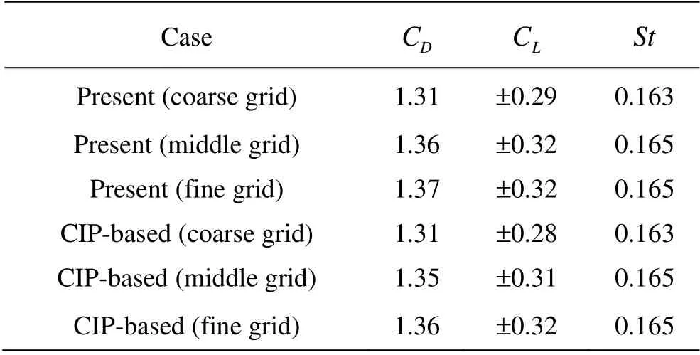
Table 4 Comparisonofresultsfromtwomodelswith different grid resolutions

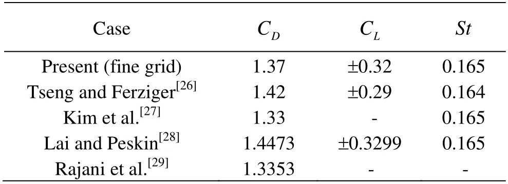
Table 5 Comparison of results from the present model with the fine grid size and existing literature data

Table 6 and Fig. 14 show the comparison of the computational time between the Tensorflow-based model and CIP-based model. It is clearly illustrated that the computational time of the TensorFlow-based model increases much more slowly than that of the CIP-based model, which is similar to the lid-driven cavity flow test above. When the grid number increases to 614 400, the CIP-based model takes more than 92 h while our TensorFlow-based model only takes about 6.77 h, in which case the computational efficiency is raised by 13.68 times. It should also be noted that with the same tolerance assigned, the present TensorFlow model is supposed to produce more precise results. Considering that different programming languages and different Poisson solvers are used, the acceleration ratio is only taken as a reference here.

Table 6 Comparisonsofthecomputationaltimeofthe TensorFlow-based model and CIP-based model

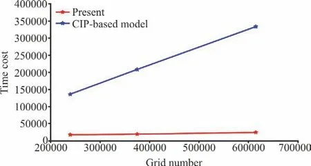
Fig. 14 (Color online) Comparisons of the computational time between the TensorFlow-based model and CIP-based model

3. Conclusion

In this paper, a new efficient CFD model is developed based on the TensorFlow framework. The CIP scheme is adopted as the base flow solver for the advection term in the N-S equations and the PCG method is used to solve the Poisson equation. Some new features including the convolution, vectorization,and GPU acceleration were implemented to raise the computational efficiency. The model was validated by several numerical tests and the results agree well with exact solutions or previous numerical results. The presented results indicate that the TensorFlow framework not only helps researchers to reduce programming work with Python, but also helps to achieve GPU acceleration easily to promote computational efficiency. Compared with our former CIP-based model, which uses the same discrete scheme but is written in Fortran, the computational time of the present model can be greatly shortened in time-consuming simulations, and the acceleration ratio increases as the grid number grows. Due to its high-performance computational ability and simplicity for programming, the TensorFlow framework might be a new choice for CFD models.

Acknowledgements

This work was supported by the Natural Science Foundation of Zhejiang Provincial (Grant No.LR16E090002), the Fundamental Research Funds for the Central Universities (Grant No. 2018QNA4041),Blue Bay Renovation Project of Pingtan Comprehensive Pilot Zone, the Bureau of Science and Technology of Zhoushan (Grant No. 2018C81040),the HPC Center OF ZJU (Zhoushan Campus) and the Tang scholar.