(1.College of Mathematics and Physics,Wenzhou University,Wenzhou 325035,China;2.School of Mathematics and Statistics,Henan University,Kaifeng 475004,China)

Abstract:We study the conjugate gradient method for solving a system of linear equations with coefficients which are measurable functions and establish the rate of convergence of this method.

Keywords:Riesz algebra;Matrices;Measurable functions;Ordered structures;Conjugate gradient methods;Computational methods in function algebras

§1.Introduction

Consider a computer program used to give numerical solutions of stochastic differential equations which are the backbones of financial mathematics today.The input data are supposed to be the values at certain points of the input random variable and the output which will also believe to be the values of the output random variable,in fact the output data points are correlated to give an random variable which is then used to calculate the values at other intermediate points.If the program used for this computation contains subroutines based on certain numerical methods which may corrupt random variables,then when we input a random variable we are no longer certain the output is still a random variable.Though we all know a trader at the desk only cares about the numbers but a quantitative analyst would certainly feel better if he knows at least theoretically that,when the input is a random variable,the computer programs do output a random variable and not just a function pretending to be an instance of a random variable.We show in this paper that a numerical computation of random variables using the conjugate gradient method is robust-input a random variable it will output a random variable.This is the raison d’?etre of this paper.We can give the same arguments for quantum mechanics where we deal with wave functions which are random variables.

Take another example-let us consider the control problem for correction of the positions of satellites.A radio command signal from an earth station in position takes 0.13 seconds to reach a communication satellite in a geostationary orbit above the equator at an altitude of 38,000 km.Thus we can say a feed back control procedure based on numerical computation by a fast computer is almostinstantaneous.This is no longer so for a landing module orbiting the moon simply because the radio signal propagation time from the Earth to the Moon is about 1.28 seconds-10 times slower than that of an earth orbiting satellite.We can extrapolate from the last observed data hoping that all our calculations actually produced a bona fide function.Even though we tend to think of all the data involved is a function describing a rigid body problem,the complexity of the entire engineering system would build in so many correction errors that it is perhaps better to consider the data of the position for example are just point values of a random variable.In that case,if we know all our numerical programs for satellite positioning actually preserve random variables so that our outputisa random variable we can proceed to calculate this random variable and not just to extrapolate-we can be ahead of the time-lag due to signal delay.For a mission to Mars,the signal distance is the largest when the Mars and the Earth are at the opposite sides of the Sun,and in this case the time needed for an radio command signal from earth to Mars is approximately 21 minutes.It is hopeless to expect an instantaneous feed back control sequence to work and your confidence level by extrapolation also drops.However if we accept that our position is a random variable and our computations preserve random variables,our output data is the random variable that actually gives the probability of the position,then we can confidently use this random variable to calculate without worrying about the signal delay.

In scientific or financial computations the relation of the input data set to the output data set is often a probability distribution or a random variable.Due to the inability to make precise measurements even the input data set is sometimes itself a random variable.So the natural question that arises is whether the standard numerical methods can take a random variable input to give a random variable output.In this paper we give a new theoretical foundation to justify a random variable approach to the most commonly used method in numerical linear algebra,namely the conjugate gradient method.

This is indeed not the first attempt at this question,in[12],[13]we have studied the preconditioning of Toeplitz systems.Recently Cheng,Fang and Zhu studied random model of non-selfadjoint,bounded linear operators in[6].

The conjugate gradient method(CGM)is one of the most important iterative methods used to solve a numerical linear systemAx=b([9],[2]).Couple with preconditioning it is often the most efficient method[5],[18].Function space analogues of the conjugate gradient methods was considered by[7],[16].

In this paper we take a different approach,we construct a new structure-a theory ofRiesz algebraand apply it to deal with measure theoretical questions when we run conjugate gradients on random variables.We shall see in the course of this paper that the Riesz algebra is not there just to be fancy but it is necessary in order to have a theory of inequalities for functions.

When the coefficient matrixAof the system is not numerical but of the formC+EwhereCis a matrix with entries in complex numbers whileEis a matrix with entries which are random variables,much work have been on the statistical analysis of such systems.

We shall go in a different direction.The goal of this paper is to study the algebraic aspects of the computation.We want to apply CGMdirectlyto a linear systemAx=bin whichA,x,bhave entries which are real valued measurable functions.From a computational point of view we are in a totally new direction.We are proposing to calculate the functions as elements of a ring and try to obtain solutions to very large systems as functions and not to evaluate the system at a few selected points,compute numerically a solution at a these selected points and pretend that these few numerical values give in fact the whole function which is the solution of the given system.As it is usual to work with measurable functions equivalent up to sets of measure zero and we need to invert strictly positive elements in order that CGM works,we replace the ring of measurable functions with a commutative real algebraRconstructed from it by taking quotient[20]and localization[4].We give an abstract characterization ofRand call it a Riesz algebra(to compare it with a similar structure[8]).In order to establish the rate of convergence of CGM by Krylov’s method in this case we shall see that we need all the rich structures of a Riesz algebra to get results on positive definite quadratic forms and min-max estimates which are standard over fields.This will show that the Riesz algebra is the right place for computational linear algebra for functions.

Professor Wong Yau Chuen(1935-1994)was an excellent functional analyst who taught at the Chinese University of Hong Kong;Professor Wong Ngai Ching was his student and he in turn taught Hsu Ming Hsiu.Lai always remember Professor Wong Yau Chuen as a good friend and colleague.We would like to thank the referee for his perspicacious reading and useful suggestions.

§2.Riesz algebra

We give the definition of a Riesz algebra.

By apartially ordered ringwe mean a ringRwith identity equipped with a partial order≤such that(1)forx,y∈R,ifx≤ythenx+a≤y+afor anya∈R,(2)ifx≥0 andy≥0 thenxy≥0 and(3)a2≥0 for alla∈R.Writea≤bifb-a≥0.We refer to[4]for more information.

Let R be the field of real numbers.A partially ordered R-algebraRis a partially ordered ring such that(1)ifa≥0 inRandαis a non-negative real number thenαa≥0(i.e.Ris a partially ordered vector space,see[8]§12),and(2)the order ofRextends that of the real numbers R.i.e.ifα≥0 is a real number and 1 is the identity inRthenα1≥0 inR.We shall writeαforα1.

Say an elementain a partially ordered ringRis positive and writea＞0 ifa≥0 anda/=0.We sayaisstrictly positiveand writea﹥0 ifa＞0 andais invertible inR.We say that a partially ordered R-algebraRisstrictly archimedeanif for anya,b∈R,the conditionrb?aholds for anyr∈R implies thatb=0.

Alatticeis a partially ordered set(A,≤)such that the supremum sup{a,b}and infinmum inf{a,b}exist for any pair of elementsa,b∈A.We write|a|for sup{a,-a}.A partially ordered ring(R,+,·)which is also a lattice is called a lattice-ordered ring([20]§3.1).A partially ordered vector space which is also a lattice is called aRiesz space([8]§14A).

Definition 2.1.We shall call a partially ordered strictly archimedeanR-algebra R which is also a lattice a Riesz algebra.If for every a﹥0in R there exists in R an element b﹥0suchthat b2=a,we say that R is a real Riesz algebra.Write b as(cf.[11]I p.308).When R isalso commutative we call it a commutative real Riesz algebra.

We say an×nsymmetric matrixAwith entries in a commutative real Riesz algebraRis positive definite if for any non zero vectoryin theR-moduleRnof columnn-vectors we haveyT Ay﹥0 inR.Forx,y∈Rnwe write〈x,y〉A(chǔ)forxT Ay.Say two vectorsx,yareconjugateorA-conjugate orAperpendicular if〈x,y〉A(chǔ)=0.Ifx/=0 put‖x‖A=and set‖0‖A=0.

Proposition 2.1.(Schwarz inequality)Let A be a positive definite symmetric matrix with entries in a commutative real Riesz algebra R.For any non zero vectors x,y∈Rn then we have in R

Proof.As‖x‖Ais inRwe have

AsAis positive definite we get 2‖x‖A‖y‖A〈x,y〉A(chǔ)?.As strictly positive elements are invertible in a Riesz algebra,2,‖x‖A,‖y‖Aare invertible and it follows that

A similar calculation of〈‖x‖Ay+‖y‖Ax,‖x‖Ay+‖y‖Ax〉A(chǔ)shows that-〈x,y〉A(chǔ)?‖x‖A‖y‖A.

Corollary 2.1.(Triangle inequality)For non zero vectors x,y∈Rn we have

We continue to writeRfor a commutative real Riesz algebra andR×for the subgroup of invertible elements inR.We have just seen that〈x,y〉A(chǔ)is a symmetric bilinear form on theR-moduleRn.In general we can consider a symmetric bilinear formb:M×M→Ron a finitely generatedR-moduleM.For a submoduleSofMwe writeb|Sfor the restriction ofbtoSand For aR-moduleMlet us write HomR(M,R)for the theR-module ofR-linear module homomorphisms fromMtoR.We say a symmetric bilinear formbon a finitely generatedR-moduleMis non-degenerate if

1.b(x,y)=0 for ally∈M?x=0,

2.iff∈HomR(M,R)then there existsxf∈Msuch thatf(y)=b(xf,y)for anyy∈M.

Just as in the case over fields it can be proved that a symmetric bilinear form on a finite rank freeR-module is non-degenerate if and only if its matrix associated to any basis is invertible.Moreover the following results are standard.

Proposition 2.2.Let b be a symmetric bilinear form on a finitely generated R-module M.Then

1.M=S⊥S⊥meaning M=S⊕S⊥and b=b|S⊕b|S⊥,that is for x,y∈S and u,v∈S⊥we have

2.Put N={x∈M:b(x,x)/∈R×}.Then N is a R-submodule of M.

3.If N/=M then there exist x1,···,xk∈M such that b(xi,xi)∈R×and

([11]I Theorem 6.1,[3],[15]).

§3.Algebra of measurable functions

We fix a measure space(X,Σ,μ);hereΣis aσ-algebra of subsets ofXand we assume thatμ(X)is finite.We write a.e.for almost everywhere.

The setMof all real valued measurable functions onXis a commutative R-algebra.The setNconsisting of functions which are zero a.e.is an ideal inM.LetRdenote the quotient ringM/N.Write〈f〉for the image off∈MinR.

Set〈f〉≥0 ifμ{f＜0}=0.ThenRis a partially ordered ring and a Riesz space(see[8]§62F(c)§62G,[20]§3.1).To say that〈f〉/=0 is sayingf/∈N,i.e.μ{f/=0}/=0.We write〈f〉＞0 to mean〈f〉≥0 and〈f〉/=0.

We shall write〈f〉﹥0 ifμ{f≤0}=0.LetSbe the set of all〈f〉inRsuch that either〈f〉﹥0 or〈-f〉﹥0.ThenSis a multiplicative set inR.We localizeSto get a ring of quotientsRin which every element inSis invertible([17]§4).We can represent an element ofRaswith〈g〉inRand〈f〉inS.We say≥0 if〈f〉〈g〉≥0.This defines a partial order makingRa partially ordered ring.Fora=we shall writea﹥0 if〈f〉〈g〉﹥0.Thena﹥0 if and only ifa＞0 andais invertible inR.

Supposea=and〈f〉﹥0.Forx∈Xwe seth(x)=0 iff(x)≤0 and equals tootherwise.Thenhis measurable([10]§11 Theorem 11.8)andh=a.e.We set sup{a,0}to be the image of sup{h,0}inR.Similar definition is given when〈-f〉﹥0.Clearly ifa∈Rthen this agrees with the definition of sup inR(as in[8]14G(c)).This defines the structure of a lattice inR.

We summarize our discussion in the following proposition.

Proposition 3.1.R is a real Riesz algebra.

From now onRwill always denote this Riesz algebra.We also sayRis the Riesz algebra on the measure spaceX.

LetAbe an×nmatrix with entries in the Riesz algebra of measurable functions on a measure spaceX.Then it is known that its eigenfunctions can be ordered[14],[1]

Proposition 3.2.Let A be a n×n positive definite symmetric matrix with entries in the Riesz algebra R on the measure space X.Letyj(in Rn)be the eigenvector of A with eigenvalueλj.Then{yj}form a basis of Rn.

Proof.IfAis positive definite then in the notation of the proposition 2.2 the spaceNassociated to the bilinear form〈·,·〉is zero.And so

Thus,we complete the proof.

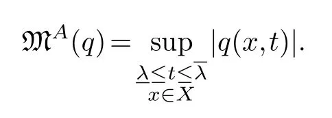
LetAbe an×npositive definite symmetric matrix with entries in the Riesz algebraRon the measure spaceX.Writeλminfor its minimal eigenfunction andλmaxfor its maximal eigenfunction.Put

Proposition 3.3.Notations as above.If q is a polynomial over R,andx∈Rn then in R we have

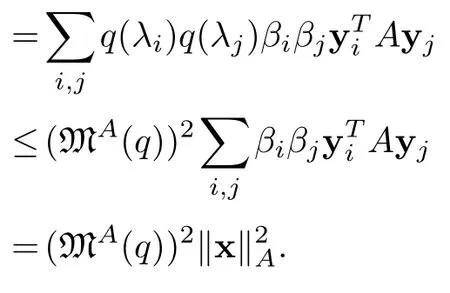
Proof.Take yjas in the previous proposition,write x=then

and

Hence,‖q(A)x‖A≤MA(q)·‖x‖A.

§4.Conjugate gradient method

LetAbe an×npositive definite symmetric matrix with entries in the Riesz algebraRon a measure spaceXand b a vector inRn.We try to find iteratively a solution x∈Rnof the linear systemAx=b.

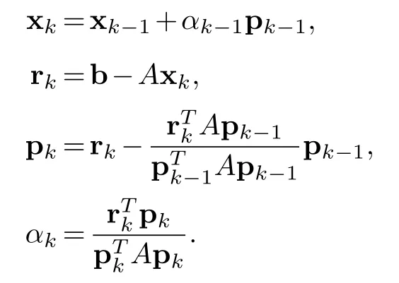
We start with any point x0inRnand take r0=p0=b-Ax0.At thek-th step we compute

The termαkis called the control term.Ifαkis in the setSof positive definite or negative definite elements we say it is acceptable and we continue.We shall also say in this case that the CGM isfeasiblefor the given system at thek-th step.Ifαkis not inSwe stop the program.The point is this.Ifαk(x)=0 atx∈Xwe can say(b-Axk)(x)=0 and we find a solution xk(x)of the systemA(x)x(b)=b(x)at the pointx.But this does not tell us if the function x gives the solution at other points in the spaceX.The problem being that the algebraRhas plenty of non-zero zero-divisors.This shows the difficulty of solving for functions.But if we do find a function solution we have a global solution rather than a solution at a point in the spaceX.This shows the convenience of working in an abstract Riesz algebra.

This computation will have a failure set

which is of measure zero by the choice ofA.As countable union of sets of measure zero has measure zero,we know that we can continue outside of∪kΥk,that is the computation of the conjugate gradient can be done a.e.

By aKrylov moduleof then×nmatrixAwe mean aR-moduleK(A,y,k)spanned overRby the set{y,Ay,···,Aky}where y is a vector inRnandkis an integer.

Theorem 4.1.In the above notations assuming that CGM is feasible for the linear systemAx=b.Then

1.=0for0≤i＜j≤k.

2.=0for i/=j,0≤i,j≤k.

3.〈pi,pj〉A(chǔ)=0for i/=j,0≤i,j≤k.

4.K(A,r0,k)is spanned by{r0,···,rk}or by{p0,···,pk}.

Proof.We prove the induction step fromktok+1.

For part(1)-from the definition of rkwe get

From this and the definition ofαkit follows that=0 and also by the induction hypothesis for parts(1)and(3),=0 for 0≤i≤k-1.

For part(2)-we get from part(1)that=0 for 0≤i≤k.By the induction hypothesis of part(4)which says that{r0,···,rk}and{p0,···,pk}span the same module,we conclude that=0 for 0≤i≤k.

For 0≤i＜kassuming that the program can continue and theαi(0≤i≤k-1)are acceptable,from part(2)proved above and by the induction hypothesis of part(3)it follows that=0.By construction=0.

For part(4)-we start with the induction hypothesis that either{r0,···,rk}or{p0,···,pk}spansK(A,r0,k).Then the formulas rk+1=rk-αkApk,and pk=rk-βkpk-1,tell us that rk+1,pk+1are inK(A,p0,k+1).

ForAkr0inK(A,r0,k)we can writewithγi∈R.ThenAk+1r0=From piinK(A,r0,k)we getApiand soAk+1r0is inK(A,r0,k+1).

Moreover parts(2)tells us that the vectors r0,···,rk+1are linearly independent so are p0,···,pk+1.ThusK(A,p0,k+1)is free of rankk+1 overR.

Remark 4.1.The theorem tells us that the CGM stops before the n+1step either when it is successful or when it is not feasible.

Proposition 4.1.In the above notations assuming that CGM is feasible for the linear system Ax=bx?.Then for k＜we have

Proof.From the construction we have xk=xk-1+αk-1pk-1.It follows that(i)xk=x0+α0p0+···+αk-1pk-1,and(ii)x?=xk+αkpk+···+α?-1p?-1.

From(i)we see that xk∈x0+K(A,r0,k-1)and so for any x∈x0+K(A,r0,k-1)we get xk-x is inK(A,r0,k-1)which is spanned by p0,···,pk-1.While(ii)says x?-xkis in the submodule spanned by pk,...,p?-1.By theorem 4.1(3)that,〈x?-xk,xk-x〉A(chǔ)=0 and so the proposition follows from

Consequently,the proof is completed.

§5.Rate of convergence

We continue to writeRfor the Riesz algebra on the measure spaceX.We are interested in the setof polynomials in the variableToverRof degree≤kwith constant term 1.Let us consider an elementp=1+a1(x)T+···+ak(x)Tkinas a function onX×[a,b]for some 0＜a＜b.Then we can consider the real valued mapMongiven by

We can apply the standard result in approximation theory at least pointwise inXto find a lower bound forM.Namely let

denotes the Chebyshev polynomial of degreek[19].And put

This is a polynomial inTwith real coefficients.Letdenote the set of polynomials over R of degree≤kwith constant term 1.For a real polynomialpwrite

Then by approximation theory([19],[2]Appendix B)we have

But

So

NowAnd forwe have M(p)=m(p).Thus

Theorem 5.1.Let A be a n×n matrix with entries in the Riesz algebra of a measure space X.Writeλminfor its minimal eigenfunction andλmaxfor its maximal eigenfunction.Put

andκ=Assume that the conjugate gradient method for the linear system Ax=bissuccessful and yields an exact solutionx*.Then the k-th feasible outputxk satisfies the followingestimate

Proof.From theorem 4.1(4)we know that for any x∈x0+K(A,r0,k-1)there exists a polynomialpk(T)inR[T]of degreek-1 such that x=x0+pk(A)r0.Recall that r0=b-Ax0.Hence

whereqk(T)=1-Tpk(T)is a polynomial of degreekandqk(0)=1.

Applying proposition 4.1 we get

Using proposition 3.3 we have

This theorem is proved.

This is the same estimate as in the numerical case as given in([2]§13.2.1).

§6.Conclusions

We have seen to what extent CGM can be used to solve a large linear system over the algebra of measurable functions on a measure space.The aim is to try to find a function which is a solution of the system rather than just doing a point-wise computation and getting only the values of the solution function at a few selected points.In the process we see that we need the theory of quadratic forms over rings and an order structure on the ring of measurable functions for estimates.The result is a Riesz algebra.It is clear that much can be done about computational linear algebra over a Riesz algebra-for example we can develop preconditioning methods for Wiener-Hopf integral equations in this context.We hope to extend the work of Lasdon,Mitter and Waren to the conjugate gradient method for optimal control problems in random variables.