Grace Nnennaya OGWO Chinedu IZUCHUKWU Oluwatosin Temitope MEWOMO

School of Mathematics,Statistics and Computer Science,University of KwaZulu-Natal,Durban,South Africa

E-mail: 219095374@stu.ukzn.ac.za;izuchukwuc@ukzn.ac.za;mewomoo@ukzn.ac.za

Abstract Many methods have been proposed in the literature for solving the split variational inequality problem.Most of these methods either require that this problem is transformed into an equivalent variational inequality problem in a product space,or that the underlying operators are co-coercive.However,it has been discovered that such product space transformation may cause some potential difficulties during implementation and its approach may not fully exploit the attractive splitting nature of the split variational inequality problem.On the other hand,the co-coercive assumption of the underlying operators would preclude the potential applications of these methods.To avoid these setbacks,we propose two new relaxed inertial methods for solving the split variational inequality problem without any product space transformation,and for which the underlying operators are freed from the restrictive co-coercive assumption.The methods proposed,involve projections onto half-spaces only,and originate from an explicit discretization of a dynamical system,which combines both the inertial and relaxation techniques in order to achieve high convergence speed.Moreover,the sequence generated by these methods is shown to converge strongly to a minimum-norm solution of the problem in real Hilbert spaces.Furthermore,numerical implementations and comparisons are given to support our theoretical findings.

Key words split variational inequality problems;relaxation technique;inertial extrapolation;minimum-norm solutions;product space formulation;half-spaces

1 Introduction

Let C and Q be nonempty closed and convex subsets of real Hilbert spaces H1and H2,respectively.LetF: H1→H1,A: H2→H2be two operators andT: H1→H2be a bounded linear operator.The Split Variational Inequality Problem (SVIP) is defined as follows:Findx∈C that solves

such thatw=T x∈Q solves

Observe that (1.1) and (1.2) are classical Variational Inequality Problems (VIPs) which have been studied by numerous researchers (see,for example,[1,4,17,18,22,29,30,49,50]).Thus,when viewed separately,the SVIP constitutes of a pair of VIPs in which one VIP have to be solved in a given space H1and its image under a given bounded linear operator is a solution of the other VIP in another given space H2.The SVIP (1.1)–(1.2) can also be seen as a combination of the classical VIP (1.1) and the split feasibility problem introduced in [12],see also [19,27].Some of the special cases of the SVIP include,the split minimization problem [37],split common null point problem [45,47] and split common fixed point problem [35].Thus,it has wide applications in different fields such as medical treatment of the Intensity-Modulated Radiation Therapy (IMRT),data compression,medical image reconstruction,signal processing,phase retrieval,among others (for more applications see [9,12,14]).

The classical VIP have been studied by many authors under the assumption that the cost operator is not co-coercive (see [11,18,50,54]) but few authors have studied the SVIP under this assumption.The first known results for SVIP is due to Censor et al.[13] (see also [14]).They studied the SVIP when the operators are monotone and Lipschitz continuous,by first transforming the problem into an equivalent Constrained VIP (CVIP) in the product space H1× H2(see [13,Section 4]) and then employed the well-known subgradient extragradient method [15] to solve it.However,the product space formulation approach has some weaknesses,which include;the potential difficulty in computing the projection onto some new product subspaces of H1× H2,the fact that it does not efficiently exploit the splitting structure of the SVIP (1.1)–(1.2) and possibly,the difficulty in translating the method back to the original spaces,H1and H2(see,for example [13,page 12]).To overcome these weaknesses,the authors further proposed a projection method which does not require any product space formulation.Hence,the projection based method was easily implemented without the difficulties possibly caused by product space formulation.This projection based method is given as: forx1∈H1,the sequence {xn} is generated by

whereT*is the adjoint ofT,Iis the identity operator,η∈(0,)withLbeing the spectral radius ofT*TandPC,PQare metric projections onto C,Q,respectively.They proved that the sequence {xn} generated by (1.3) converges weakly to a solution of the SVIP (1.1)–(1.2) under the assumptions that,the solution set of problem (1.1)–(1.2) is nonempty,A,FareL1,L2-cocoercive operators,respectively,λ∈[0,2α],whereα:=min{L1,L2},and for allxwhich are solutions of (1.1),the following holds

Observe that even though Algorithm (1.3) fully utilizes the important splitting structure of the SVIP (1.1)–(1.2) and does not require the product space formulation,the weak convergence of this method requires some strong assumptions,which are the facts that both operators are required to be co-coercive and assumption (1.4) needs to hold.

Recently,He et al.[20] proposed a novel approach (given in Appendix 6.1) for solving the SVIP (1.1)–(1.2),whenAandFare monotone and Lipschitz continuous in finite dimensional spaces.This approach is based on decomposition techniques and it fully utilizes the splitting structure of the SVIP.However,this method has some weaknesses since it requires the problem to be reformed into an equivalent VIP in a product space.

In recent literature,few authors have attempted to solve the SVIP (1.1)–(1.2) in real Hilbert spaces without reformulating the problem into some VIPs in a product space.However,The methods proposed by these authors have some limitations.For example,Tian and Jiang [55]proposed a viscosity method ([55,Algorithm (3.1)]) for solving a certain class of generalized split feasibility problems ([55,problem (1.10)]) in real Hilbert spaces.They applied their method to the method given in Appendix 6.3,to solve the SVIP (1.1)–(1.2),whenAis monotone and Lipschitz continuous butFis required to be co-coercive,which is generally known to be limited in many applications.A similar method was also used to solve problem (1.1)–(1.2) in [56,Theorem 3.3].Recently,Reich and Tuyen [47,Theorem 4.4] proposed a method for solving the SVIP (1.1)–(1.2) whenAandFare monotone and hemicontinuous operators.However,since their method (given in Appendix 6.2) is a hybrid projection-type,it requires the computation of three subsets and the computation of projection of an initial point onto the intersection of these subsets at each step of the iteration process;which in practice,maybe a difficult task to accomplish.Other methods for solving the SVIP (1.1)–(1.2) and its generalizations (the split monotone variational inclusion,split nonconvex variational inequality and split quasi-variational inequality problems),can be found in [16,28,32,33,36,40,51,52],which were still built up under the restrictive co-coercive assumption onAandF.Thus precluding the use of these methods in many applications.

To accelerate the convergence of iterative methods for solving the SVIP (1.1)–(1.2) and other related optimization problems,there exist different modifications of these methods.In this paper,we consider the two very important modifications,namely;inertial and relaxation techniques.The inertial technique is based upon a discrete analogue of a second order dissipative dynamical system and known for its efficiency in improving the convergence rate of iterative methods,see [2,3,31,41,43,44].The method was first considered in [46] for solving the smooth convex minimization problems.It was later made very popular by Nesterov’s acceleration gradient method [38],and was further developed by Beck and Teboulle in the case of structured convex minimization problem [8].On the other hand,the relaxation technique has proven to be an essential ingredient in the resolution of optimization problems due to the improved convergence rate that it contribute to iterative schemes.Moreover,both the inertial and relaxation techniques naturally come from an explicit discretization of a dynamical system in time.For instance,consider the following dynamical system (see,for example [7,58]):

whereθ ＞0.Using an explicit discretization of the system (1.5) in timetwith a time stepsizehn＞0 and settingxn=x(tn),γn=γ(tn),λn=λ(tn),we derive the following scheme:

wherewnis a point belonging to the line passing throughxn-1andxn(see,for example [7]).Rearranging (1.6) and settingαn=1 -γnhn,we obtain

whereV(wn)=wn-PC(wn-λnAwn) -λnAwn+λnA(PC(wn-λnAwn)).

Now,by the classical Nesterov’s extrapolation choice forwn(see also Attouch and Cabot[7]),namelywn=xn+αn(xn-xn-1),and by settingyn=PC(wn-λnAwn),we obtain after some simple simplification,that

Thus,this dynamical approach leads to the following Relaxed Inertial Tseng’s Forward-Backward-Forward (RITFBF) with parameter,?n≥1 (see,for example [7]):

Whenφn=1 andαn=0 for alln≥1,Algorithm (1.7) reduces to the well-known Tseng’s forward-backward-forward method [57],which is known to converge weakly to a solution of the classical VIP.

Given the importance of these two techniques (inertial and relaxation),it is of interest to consider their combination for solving optimization problems.Some authors have already considered incorporating these two techniques into known methods in order to achieve high convergence speed of the resulting methods.For example,in [5,6],Attouch and Cabot employed both techniques into proximal algorithms (resulting to Relaxed Inertial Proximal Algorithms(RIPA)) for solving convex minimization and null point problems.Also,Iutzeler and Hendrickx[26] studied the influence of inertial and relaxation techniques on the numerical performance of iterative schemes.

Motivated by the above research trend,our interest in this paper is to introduce two iterative methods,developed from the RITFBF (1.7) for solving the SVIP (1.1)–(1.2) in real Hilbert spaces,without any product space formulation.Our proposed methods have the following important properties:

· The proposed methods of this paper,originate from an explicit discretization of a dynamical system,which combines both the inertial and relaxation techniques in order to achieve high convergence speed.

· Our methods efficiently and fully utilizes the important splitting structure of the SVIP(1.1)–(1.2),and do not require any product space reformulation of the original problem.Thus,overcoming any potential difficulties which may be caused by product space formulation.

· In contrast to the methods in [28,32,36,51,55],whereAandFare required to be cocoercive,our proposed methods require the underlying operators to be monotone and Lipschitz continuous.Thus,our methods are potentially more applicable than these methods.

· Different from all existing methods for solving the SVIP,our methods involve projections onto half-spaces only,without any other projection onto feasible sets.Note that while projections onto feasible sets may be difficult to execute,projections onto half-spaces have closed formulas,and hence,they are easy to execute.Thus,our methods seem to be more implementable than existing ones in the literature,as shown in our numerical experiments.

· The sequence generated by the proposed methods converge strongly to a minimumnorm solution of the SVIP in real Hilbert spaces.Note that in many practical problems with physical and engineering backgrounds,it is very important if the minimum-norm solutions of such problems can be found (see for example,[20,Section 5] and [10,59]).

Organization of the paper: Section 2 contains basic definitions and results needed in subsequent sections.In Section 3,we present and discuss the proposed methods.The convergence analysis of these methods are investigated in Section 4.In Section 5,we perform some numerical analysis of our methods in comparison with other state-of-the-art methods for solving the SVIP.We then conclude in Section 6.

2 Preliminaries

In this section,we recall some definitions and results needed in subsequent sections.Throughout this section,we assume that H is a real Hilbert space with inner product 〈·,·〉,and associated norm || · ||,?x∈H.Also,we denote strong and weak convergence by “→” and “?”,respectively.

Definition 2.1LetA: H →H be a mapping.Then,Ais said to be

(i)L-Lipschitz continuous,if there exists a constantL ＞0 such that

(ii)L-co-coercive (orL-inverse strongly monotone),if there existsL ＞0 such that

(iii) monotone,if

Clearly,L-co-coercive operators are-Lipschitz continuous and monotone but the converse is not always true.

We,recall that for a nonempty closed and convex subset C of H,the metric projection denoted byPC,is a map defined on H onto C which assigns to eachx∈H,the unique point in C,denoted byPCxsuch that

It is generally known thatPCis characterized by the inequality 〈x-PCx,y-PCx〉 ≤0,?y∈C,see [39,42].

Definition 2.2A functionc: H →R is said to beateaux differential atx∈H,if there exists an element denoted byc′(x) ∈H such that

wherec′(x) is called theateaux differential ofcatx.We say that if for eachx∈H,cisateaux differentiable atx,thencisateaux differentiable on H.

Definition 2.3A functionc: H →R is called convex,if for allt∈[0,1] andx,y∈H,

Definition 2.4A convex functionc: H →R is said to be subdifferentiable at a pointx∈H if the set

is nonempty,where each element in?c(x) is called a subgradient ofcatx,?c(x) is called the subdifferential ofcatxand the inequality in (2.1) is called the subdifferential inequality ofcatx.We say thatcis subdifferentiable on H ifcis subdifferentiable at eachx∈H.

We also note that ifcisateaux differentiable atx,thencis subdifferentiable atx,and?c(x)={c′(x)}.

Lemma 2.5([60,Theorem 4.1]) Assume that the solution setV I(A,C) of the classical VIP (1.1) is nonempty and C is defined as C :={x∈H |c(x) ≤0},wherec: H →R is a continuously differential convex function.Letp∈C.Then,p∈V I(A,C) if and only if either

(i)Ap=0,or

(ii)p∈?C and there existsρ ＞0 such thatAp=-ρc′(p),where?C denotes the boundary of C.

Lemma 2.6([53]) Assume thatA: H →H is a continuous and monotone operator.Then,xis a solution of the classical VIP (1.1) if and only ifxis a solution of the following problem:

Findx∈C such that

Lemma 2.7The following are well-known in a real Hilbert space H.

(1) 2〈x,y〉=‖x‖2+‖y‖2-‖x-y‖2=‖x+y‖2-‖x‖2-‖y‖2,?x,y∈H;

(2) ‖αx+(1 -α)y‖2=α‖x‖2+(1 -α)‖y‖2-α(1 -α)‖x-y‖2,?x,y∈H,α∈(0,1);

(3) ‖x-y‖2≤‖x‖2+2〈y,x-y〉,?x,y∈H.

Lemma 2.8([48]) Let {an} be a sequence of nonnegative real numbers,{γn} be a sequence in (0,1) with conditionand {dn} be a sequence of real numbers.Assume that

Lemma 2.9([34]) Let {an} be a sequence of nonnegative real numbers satisfying the following

where {βn} is a sequnece in (0,1) and {τn} is a real sequence.Suppose thatandτn≤βnMfor someM ＞0.Then,{an} is a bounded sequence.

3 Proposed Methods

In this section,we present our proposed methods and discuss their features.We begin with the following assumptions under which our strong convergent results are obtained.

Assumption 3.1Suppose that the following conditions hold:

(a) The feasible sets C and Q are nonempty closed and convex subsets of the real Hilbert spaces H1and H2,respectively.

(b) The sets C and Q are defined as

wherec: H1→R andq: H2→R are continuously differentiable convex functions such thatc′(·) andq′(·) are Lipschitz continuous with constantsK1andK2,respectively.

(c)A: H1→H1andF: H2→H2are monotone and Lipschitz continuous with Lipschitz constantsL1andL2,respectively.

(d)T: H1→H2is a bounded linear operator and the solution set Γ :={z∈V I(A,C) :T z∈V I(F,Q)} of the SVIP (1.1)–(1.2) is nonempty,whereV I(A,C) is the solution set of the classical VIP (1.1).

We present the following method for solving the SVIP (1.1)–(1.2) whenL1,L2,K1andK2are known.

Algorithm 3.2Relaxed inertial method with fixed stepsizes.

Step 0Choose sequencessuch that the conditions from Assumption 3.1 (e) hold and letη≥0,φ∈(0,1],α≥3 andx0,x1∈H1be given arbitrarily.Setn:=1.

Step 1Given the iteratesxn-1andxn(n≥1),chooseαnsuch that 0 ≤αn≤n,where

Step 2Compute

Step 3Compute

Step 4Construct the half spaceStep 5Compute

Setn:=n+1 and go back to Step 1.

In the case where the Lipschitz constantsL1,L2,K1andK2are not known,we present the following method with adaptive stepsizes for solving the SVIP (1.1)–(1.2).

Algorithm 3.3Relaxed inertial method with adaptive stepsize strategy.

Step 1Given the iteratesxn-1andxnfor eachn≥1,chooseαnsuch that 0 ≤αn≤n,where

Step 2Compute

Step 3Compute

Step 4Construct the half-space

Step 5Compute

Setn:=n+1 and go back to Step 1.

Remark 3.4· Observe that Algorithms 3.2 and 3.3 can be viewed as modified RITFBF(1.7),involving only one projection onto the half-space Cnper iteration for solving the classical VIP in H1and another RITFBF involving one projection onto the half-space Qnper iteration under a bounded linear operatorTfor solving another VIP in another space H2,without projections onto feasible sets,unlike other existing methods for solving SVIPs,where projections onto feasible sets are required;for instance,the method in [18,50] for the case of classical VIP.A notable advantage of these methods (our algorithms) is that the co-coercive assumption on the operatorsAandFusually used in many papers (see for example,[28,32]) to guarantee convergence is dispensed with,and no product space formulation of any sort is required under this setting,unlike in [13,20].

· The stepsizes {λn} and {μn} given by (3.5) and (3.6),respectively are generated at each iteration by some simple computations.Thus,Algorithm 3.3 is easily implemented without the prior knowledge of the Lipschitz constantsL1,L2,K1andK2unlike in [18,Algorithm 4.1]where the knowledge of the Lipschitz constant is required and [50,Algorithm 3.3] where the stepsize is assumed to be 1.

· Step 1 of our methods is also easily implemented since the value of ||xn-xn-1|| is a prior known before choosingαn.

· Step 5 of both algorithms guarantee the strong convergence to the minimum-norm solution of the SVIP .

· It is easy to see that Cn?C and Qn?Q.Furthermore,since Cnand Qnare half-spaces,the projections onto them have explicit formulas.In fact,unandynin our methods can be calculated as:

Hence,our methods are computationally less expensive than other existing methods for solving the SVIP (1.1)–(1.2).This benefit (brought by the half-spaces) is further verified in our numerical analysis.

Remark 3.5The choice of the stepsizeηnin Step 3 of Algorithms 3.2 and 3.3 do not require the prior knowledge of the operator norm ‖T‖,unlike in [13,20,36,55].Note that algorithms whose implementation depends on the operator norm require the computation of the norm of the bounded linear operator,which in general is a very difficult task to accomplish as shown in [24,Theorem 2.3].

Also,we note that the value of the constantηin our methods does not influence the algorithms,but it was introduced for the sake of clarity.In what follows,we show thatηnis well-defined,and then,present an alternative choice forηnwithout involving the constantη.

Proposition 3.6The stepsizeηngiven in Step 3 of Algorithm 3.2 (or Algorithm 3.3) is well-defined.

ProofLetz∈Γ.Then,by Lemma 2.7 (1),we obtain

We shall prove this claim (inequality (3.10)) later in Lemma 4.1 without involving the stepsizeηn.

Now,by the condition onλ,that is,from (3.2),we obtain

By some simple simplifications,we get

SinceL2,φ ＞0,dividing through by,we obtain

which implies that

Hence,we obtain from (3.10) that

Note that ifλis replaced withλnas in Algorithm 3.3,we will use inequality (4.52) (instead of(3.10)) and relation (4.54) (instead of (3.11)) to get (3.12).Therefore,substituting (3.12) into(3.9),we obtain that

Now,forznT wn,we have that ‖T wn-zn‖＞0.This together with (3.13),imply that‖T*(T wn-zn)‖‖wn-z‖＞0.Hence,we have that ‖T*(T wn-zn)‖0.Therefore,ηnis well-defined. □

We now give an alternative way of choosing the stepsizeηnin our methods.First,observe from Step 3 of Algorithms 3.2 and 3.3,that

which implies that

Thus,ηncan be chosen such that for small enough∈＞0,

Then,we can see that

which implies that

This further gives (3.14) and consequently (3.15).

As we shall see in our convergence analysis,(3.14) and (3.15) play crucial role in our proofs.Therefore,one can either choose the stepsize in Step 3 or that in (3.16),to ensure the convergence of Algorithms 3.2 and 3.3.

4 Convergence Analysis

Lemma 4.1Let {xn} be a sequence generated by Algorithm 3.2 under Assumption 3.1.Then

for allp∈Γ,whereρ1,ρ2are positive constants.

ProofLetp∈Γ.ThenT p∈V I(F,Q) ?Q ?Qn.Sinceyn=PQn(T wn-λFT wn) andT p∈Qn,we obtain from the characteristic property ofPQn,that

Also,from Lemma 2.7 (1),we obtain that

Again,sinceFis monotone,we obtain that

Substituting (4.4) and (4.5) into (4.3),we obtain

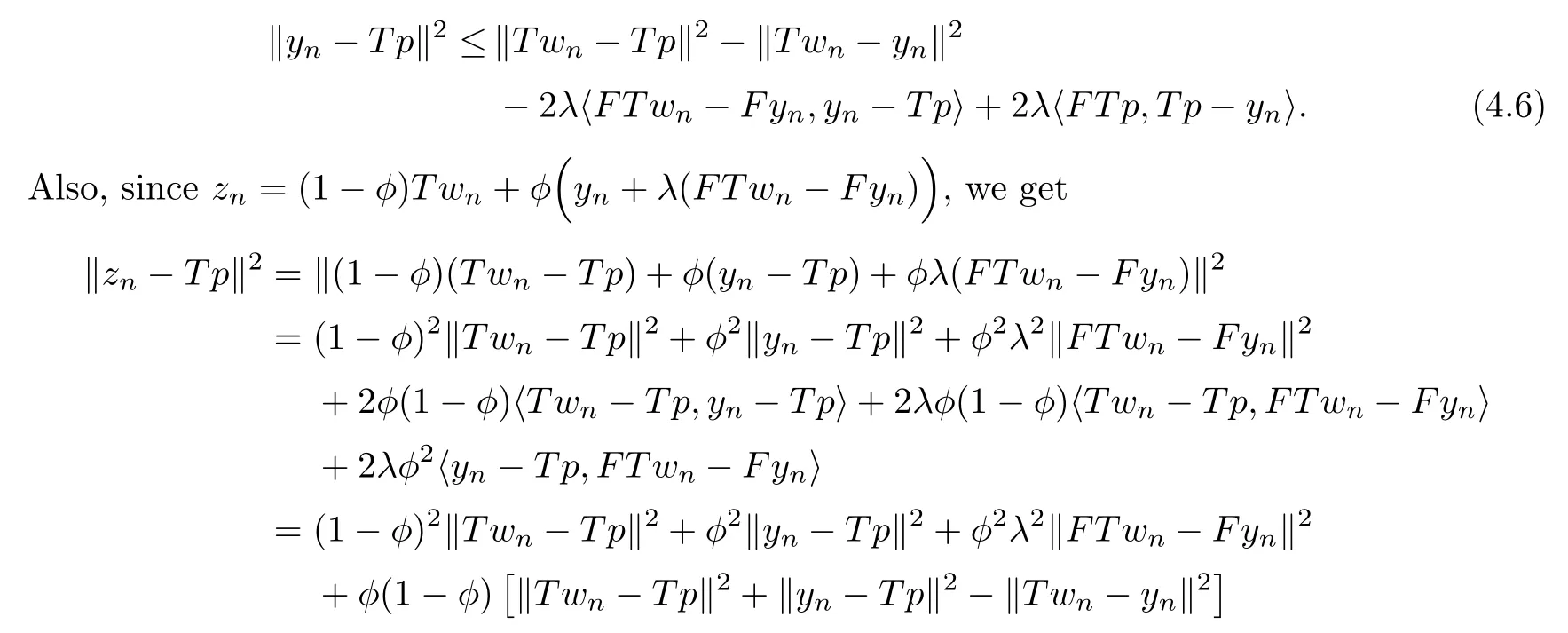
Substituting (4.6) into (4.7),we obtain

Now,ifFT p=0,then we obtain the desired conclusion from (4.9).

However,ifFT p≠0,then we obtain from Lemma 2.5 thatT p∈?Qand there existsρ2＞0 such thatFT p=-ρ2q′(T p).SinceT p∈?Q,q(T p)=0.

Also,sinceqis a differentiable convex function,it follows from (2.1) that

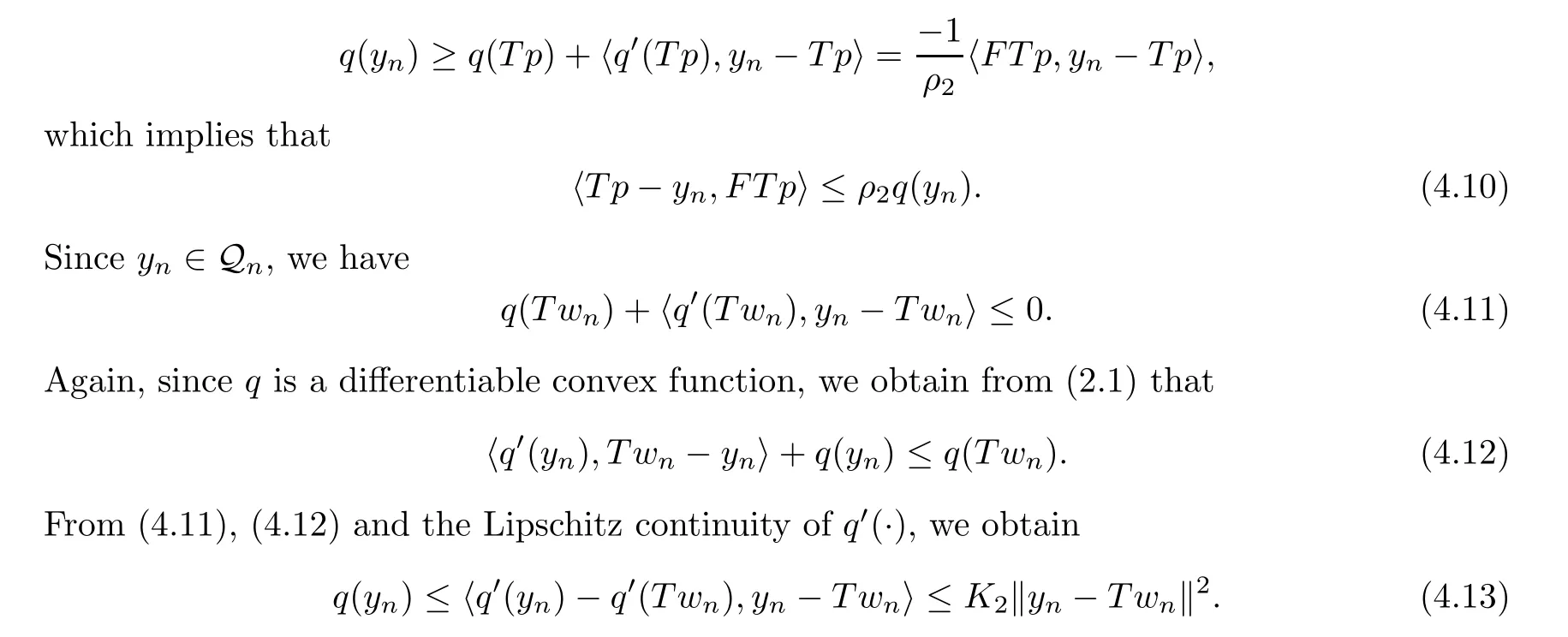
By substituting (4.10) and (4.13) into (4.9),we obtain the desired conclusion (4.1).

Following the same line of argument,we obtain (4.2). □

Lemma 4.2Let {xn} be a sequence generated by Algorithm 3.2 under Assumption 3.1.Then,{xn} is bounded.

ProofLetp∈Γ.Sincewn=xn+αn(xn-xn-1),we have

Also,from Step 1,we observe thatαn‖xn-xn-1‖ ≤τn,?n≥1,which implies that

Hence,there existsM1＞0 such that

Now,by Lemma 4.1 (inequality (4.1)) and (3.11),we obtain that

From Step 3,Lemma 2.7 and (4.17),we obtain

Thus,by the condition onηn,that is,from (3.14),we obtain that

which implies from (4.16) that

From Step 5,we have

But from (4.2),condition (3.3) and (4.19),we get that

Hence,(4.20) becomes

which implies from Lemma 2.9 that {xn} is bounded. □

Lemma 4.3Let {xn} be a sequence generated by Algorithm 3.2 under Assumption 3.1.Suppose that there exists a subsequence {xnk} of {xn} which converges weakly to a pointz∈H1andThenz∈Γ.

ProofFrom Step 2 and (4.14),we get that

Since the subsequence {xnk} of {xn} is weakly convergent to a pointz∈H1,it follows that the subsequence {wnk} of {wn} is also weakly convergent toz∈H1.This,together with our hypothesis imply that {bnk} converges weakly toz.Again,sinceTis a bounded linear operator,we obtain that {T wnk} converges weakly toT z.

Now,without loss of generality,we may assume thatzn≠T wn.

Thus,by our hypothesis,we obtain

From (4.18) and (4.24),we obtain

Sinceηnk≥∈＞0,we get that

From (4.1),we obtain

Thus,taking limit ask→∞in the previous inequality,we obtain from (4.25) and (3.11) that

Now,by the monotonicity ofF,the characteristic property ofPQnand Q ?Qn,we obtain for allw∈Q that

Thus,passing limit ask→∞in the previous inequality,we obtain

and from Lemma 2.6,we have thatT z∈V I(F,Q).

Again,by our hypothesis and (4.2),we obtain that

which by condition (3.3),implies that

Similar to (4.27),we obtain from the monotonicity ofA,the characteristic property ofPCnand C ?Cn,that

Passing limit ask→∞in the previous inequality,we obtain from (4.28) that

Therefore,we obtain from Lemma 2.6 thatz∈V I(A,C).Hence,z∈Γ.□

We now present the first theorem of this paper.

Theorem 4.4Let {xn} be a sequence generated by Algorithm 3.2 under Assumption 3.1.Then,{xn} converges strongly top∈Γ,where ‖p‖=min{‖z‖ :z∈Γ}.

ProofLetp∈Γ.Then,from Step 2,we obtain

for someM2＞0.Thus,from (4.19),(4.2) and (4.29),we get

From Step 5,the previous inequality and (4.14),we get

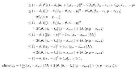
According to Lemma 2.8,to conclude our proof,it suffices to show thatfor every subsequence {‖xnk-p‖} of {‖xn-p‖} satisfying the condition;

Now,observe that

Then,from Step 5,(4.32) and (4.2),we get

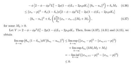
This implies that

SinceAis Lipschitz continuous on H1,we obtain from (4.38) that

Also,from Step 5,we have that

which implies from (4.38) and (4.39) that

From (4.35) and (4.23),we obtain

which implies from (4.29) that

Hence,by Step 3,we obtain

From Step 5 and (4.40),we get

From (4.42) and (4.43),we get

From (4.22) and (4.44),we get

By Lemma 4.2,there exists a subsequence {xnkj} of {xnk} which converges weakly toz,and such that

Also,since we have established (4.40) and (4.42),we can apply Lemma 4.3 to get thatz∈Γ.Note also thatp=PΓ0.Thus,we obtain from the previous inequality that

which together with (4.45),imply that

Remark 4.5· We observe that if we set H1=H2=H,F=0 andT=IH(the identity operator on H) in Algorithm 3.2,we obtain as a corollary,a relaxed inertial Tseng’s forwardbackward-forward with fixed stepsizes,involving only one projection onto the half-space Cnper iteration,for solving the classical VIP (1.1) whenAis monotone and Lipschitz continuous.This method for solving the classical VIP (1.1) is also the first in the literature.

· The conclusion of Theorem 4.4 still holds even if the fixed stepsizesλandμgiven by(3.2) and (3.3),respectively,are replaced with variable stepsizesμnandλn,respectively such that

Having concluded the convergence analysis of the first method of this paper,we now study the convergence analysis of the second method (Algorithm 3.3),which do not depend on the availability of the Lipschitz constants.We begin with the following useful remarks and lemmas.

Remark 4.6The stepsizes {λn} and {μn} generated by Algorithm 3.3 are monotonically non-increasing sequences with lower bounds minrespectively.

Indeed,it is obvious thatλn+1≤λn,?n∈N.Also,sinceFisL2-Lipschitz continuous andq′isK2-Lipschitz continuous,we get in the case where ‖F(xiàn)T wn-Fyn‖2+‖q′(T wn)-q′(yn)‖2≠0 that

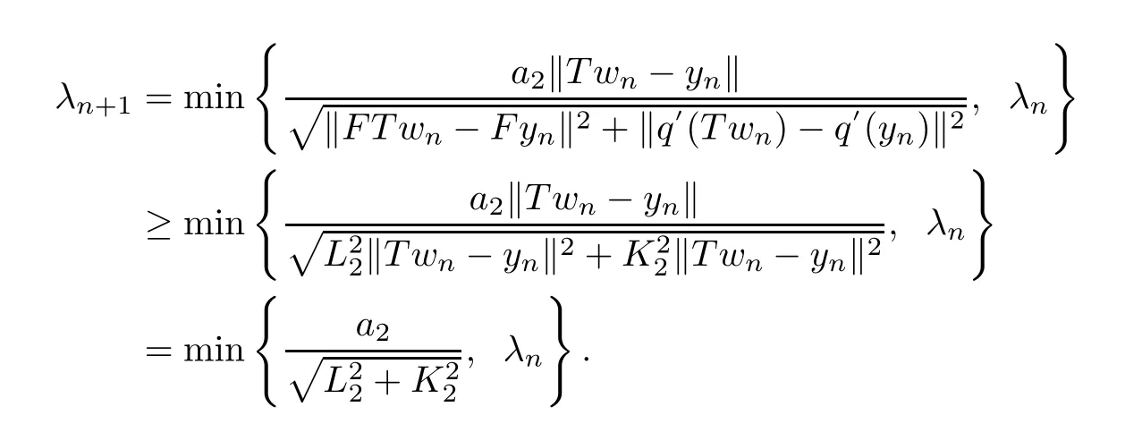
Hence,by induction,we obtain that {λn} is bounded below by min.Similar argument holds for {μn}.

Note that Remark 4.6 implies that the limits of {λn},{μn} exist,and

Remark 4.7From (3.5),we observe that

holds for both ‖F(xiàn)T wn-Fyn‖+‖q′(T wn) -q′(yn)‖0 and otherwise.This implies that

which further implies

Lemma 4.8Let {xn} be a sequence generated by Algorithm 3.3 under Assumption 3.1.Then,for allp∈Γ,there existsn0≥1 such that

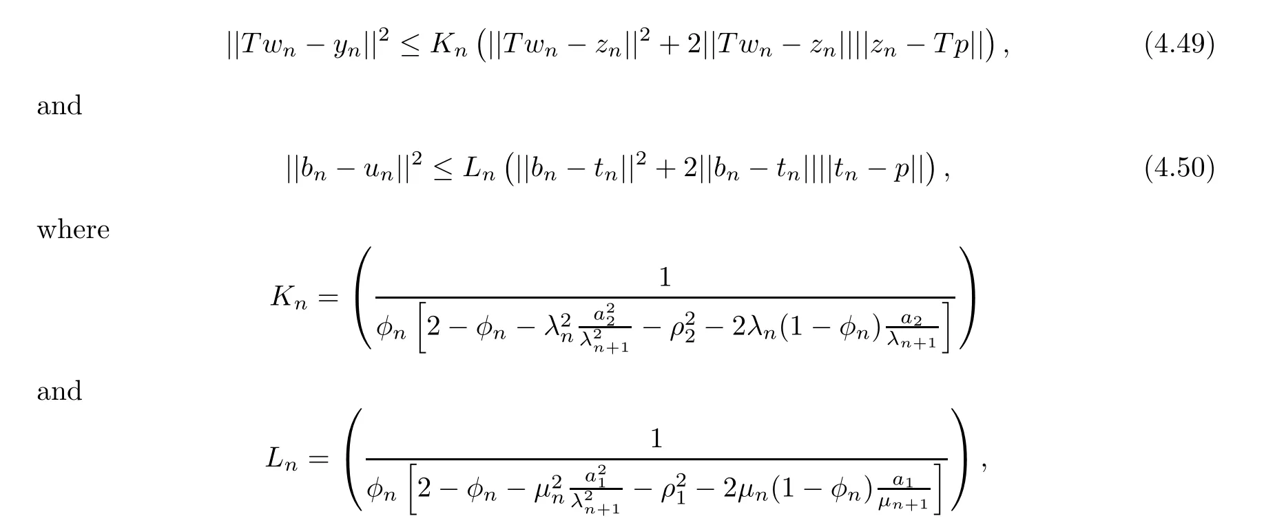
withρ1,ρ2been positive constants,for alln≥n0.

ProofBy replacingλwithλnandφwithφnin (4.8),we have

SupposeFT p=0.Then,we obtain from (4.48) and (4.51) that

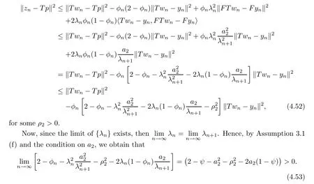
Thus,there existsn0≥1 such that

Hence,we obtain from (4.52) that

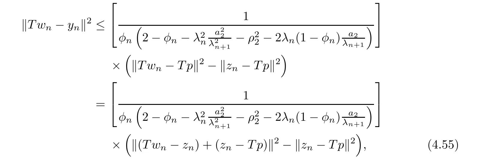
for alln≥n0,which by some simple simplifications,gives (4.49).

Now,supposeFT p≠0.Then,from (4.10) and (4.13),we obtain

Also,observe that

Substituting (4.56) and (4.57) into (4.51),and using (4.48) and (4.47),we obtain

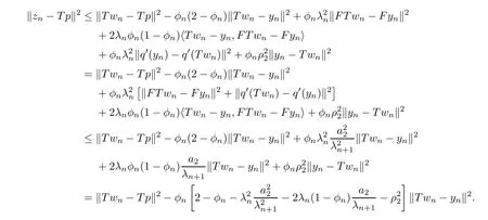
Notice that this is the same as (4.52).Hence,we obtain (4.49).

Also,we can follow the same line of proof as above to establish (4.50). □

We now state and prove the strong convergence theorem for Algorithm 3.3.

Theorem 4.9Let {xn} be a sequence generated by Algorithm 3.3 under Assumption 3.1.Then,{xn} converges strongly top∈Γ,where ‖p‖=min{‖z‖ :z∈Γ}.

ProofLetp∈Γ.Then,by replacingμandλwithμnandλn,respectively in Lemma 4.2,and using (4.52) and (4.54),we can easily get that {xn} is bounded.Furthermore,we can follow the same argument as in the proof of Theorem 4.4 to obtain (4.40),(4.41) and (4.42).Also,using (4.41) and (4.42),we can get (4.25).

Hence,from (4.25),Lemma 4.8 (that is,(4.49)) and (4.53),we obtain that

In a similar way,we can show that

Following the same arguments as in Lemma 4.3 and Theorem 4.4,we obtain the rest of the proof. □

Remark 4.10(1) Similar to Remark 4.5,we obtain a relaxed inertial Tseng’s forwardbackward-forward with adaptive stepsizes,involving only one projection onto the half-space Cnper iteration,for solving the classical VIP (1.1) whenAis monotone and Lipschitz continuous as a corollary.This method is also new.

(2) Our proofs are independent of the usual “Two cases Approach” which have been used widely in many papers (see,for example,[18,50,55]) to guarantee strong convergence of iterative methods.Hence,the techniques used in obtaining our strong convergence analysis are new for solving the SVIP (1.1)–(1.2).

(3) If Step 1 of Algorithm 3.2 and Algorithm 3.3 are replaced with the following: 0 ≤αn≤n,where

withα∈[0,1),we still have valid conclusions of Theorem 4.4 and Theorem 4.9.

5 Numerical Experiments

In this section,using various test examples,we discuss the numerical behavior of Algorithm 3.2 and Algorithm 3.3,and we compare them with the methods of He et al.[20,Algorithm 1](see Appendix 6.1),Reich and Tuyen [47,Theorem 4.4] (see Appendix 6.2) and Tian and Jiang[55,Algorithm (4.8)] (see Appendix 6.3).

We perform all implementations using Matlab 2016 (b),installed on a personal computer with Intel(R) Core(TM) i5-2600 CPU@2.30GHz and 8.00 Gb-RAM running on Windows 10 operating system.In Tables 1–3,“Iter.” means the number of iterations while “CPU” means the CPU time in seconds.

In our computations,we randomly choose the relaxation stepsizeφ∈(0,1] and the starting pointsx0,x1∈H1(see the cases below).We also choose randomly,the parametersη≥0,λ1＞0 andμ1＞0 (the choices of these parameters will be discussed in Remark 5.4).We chooseand different choices ofα:=3,6,9,12,15,which we will discuss in detail in our numerical analysis.Furthermore,in the implementation,we define,and use the stopping criterion TOLn＜εfor the iterative processes,whereεis the predetermined error.

Firstly,we consider two examples in finite dimensional spaces.In these examples,we compare Algorithm 3.2 with the method of He et al.[20] since their method is given in finite dimension spaces.

Example 5.1Consider the following separable,convex and quadratic programming problem,which has been considered by [20,Example 5.2] for their numerical experiments.

Problem (5.1) can also be rewritten as the SVIP (1.1)–(1.2),where

As done in He et al.[20,Example 5.2],we choose=104,qi=0,i=1,2 and uniformly take the vectorvi∈RNi(i=1,2) in (-1,1).In this case,AandFare monotone and Lipschitz continuous operators withLi=||Mi||,i=1,2 (which can be computed in Matlab).Furthermore,we generate the bounded linear operatorT∈RM×Nwith independent Gaussian components distributed in the interval (0,1),and then normalize each column ofTwith the unit norm.

Now,consider an ellipsoid in RNas the feasible set C.That is,C={x∈RN: (x-d)TP(xd) ≤r2},wherePis a positive definite matrix,d∈RNandr ＞0.Then,the projection onto C is difficult to compute (see,for example [21]).Consider the convex functionc: RN→R defined by,?x∈RN.Then,C is a level set ofc.That is,C :={x∈RN:c(x) ≤0}.Also,it is easy to see thatcis differentiable on RN.In fact,c′(x)=P(x-d),?x∈RN.Hence,c′isK1-Lipschitz continuous withK1=||P||.

Now,letλmaxandλminbe maximum and minimum eigenvalues ofP,respectively.

Let Q={y∈Rm:q(y) ≤0},whereThen,the explicit expression for projection onto Q may be difficult to find (see for example,[23]).Also,we note thatqis a countinuously differentiable convex function,andq′isK2-Lipschitz continuous withK2=2.Moreover,ρ2=||M2|| (see [23]).Since the Lipschitz constantsL1,L2,K1,K2are known and we knowρ1,ρ2,we can choose in Algorithm 3.2,and take the starting pointx1=(1,1,···,1)Twhile the entries ofx0are randomly generated in [0,1].

For Algorithm 1 of He et al.[20],we take

v=0.8,,γ=1.2 andρ1=-1.5 (which is the optimum choice in their implementation),with starting pointsx1=(1,1,···,1)T,y1=(0,0,···,0)Tandλ1=(0,0,···,0)T.SincePCandPQseem not to have explicit expressions,Algorithm 1 of He et al.[20] may be difficult to implement for this example.Therefore,we use the technique proposed in this paper,that is,we replace C and Q in their algorithm with Cnand Qn,then use the formulas similar to (3.7) and (3.8) for the implementation.Furthermore,we consider different scenarios of the problem’s dimensions.That is,N=100,300,500,1000 andm=N/2.We also takeε=10-6for the stopping criterion and obtain the numerical results reported in Table 1 and Figure 1.We stress that these choices are the same as in He et al.[20,Example 5.2].

Table 1 Numerical results for Example 5.1 with ε=10-6

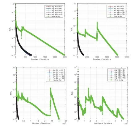
Figure 1 The behavior of TOLn with ε=10-6 for Example 5.1:Top Left: (N,m)=(100,50);Top Right: (N,m)=(300,150);Bottom Left: (N,m)=(500,250);Bottom Right: (N,m)=(1000,500)

Then,one can easily verify thatAlso,it is easy to see thatcandqare continuously differentiable convex functions with Lipschitz constantsK1=K2=2.Moreover,we have that(see for example,[23]).Furthermore,we choose the same parameters as in Example 5.1 and use the stopping criterionε=10-3.

By considering the following cases for the numerical experiments,we obtain the numerical results displayed in Table 2 and Figure 2.

Table 2 Numerical results for Example 5.2 with ε=10-3

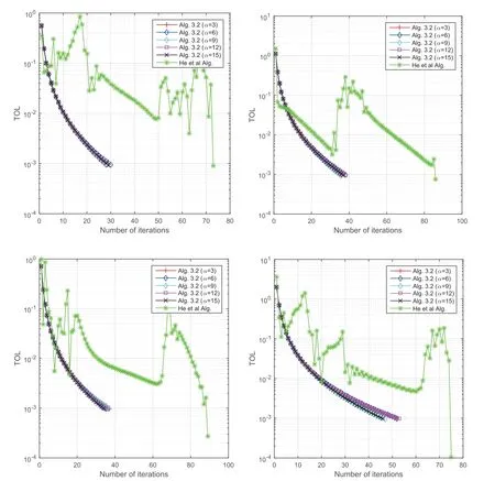
Figure 2 The behavior of TOLn with ε=10-3 for Example 5.2:Top Left: Case 1;Top Right: Case 2;Bottom Left: Case 3;Bottom Right: Case 4

Case 1Takex1=(1,0.5)Tandx0=(2,3)T.

Case 2Takex1=(2,1)Tandx0=(0.5,-1)T.

Case 3Takex1=(1,-1)Tandx0=(2,-2)T.

Case 4Takex1=(0.5,4)Tandx0=(-1,-3)T.

We present the next example in an infinite dimensional Hilbert space.In this example,we compare Algorithm 3.3 with the methods of Reich and Tuyen [47] and Tian and Jiang [55],since their methods are given in infinite dimensional Hilbert spaces.

Example 5.3Let H1=H2=L2([0,1]) be endowed with inner product

Letφbe an arbitrary fixed element in C([0,1]) (the space of all real-valued continuous functions on [0,1]) and C=Q={x∈L2([0,1]): ‖φx‖ ≤1}.In particular,for allt∈[0,1],we defineφ(t)=e-tfor C andφ(t)=e-5tfor Q.Then,C and Q are nonempty closed and convex subsets of L2([0,1]).However,we know from [21] that the explicit formulas for projections onto C and Q may be difficult to find.

Now,letc,q: L2([0,1]) →R be defined by,?x∈L2([0,1]),whereφ(t)=e-tforcandφ(t)=e-5tforq;t∈[0,1].Then,c,qare convex functions with C and Q being level sets ofcandq,respectively.Also,candqare differentiable on L2([0,1]).In fact,c′(x)=φ2x,?x∈L2([0,1]).Furthermore,c′andq′are Lipschitz continuous.

Now,defineA: L2([0,1]) →L2([0,1]) byAx(t)=max{0,x(t)},?x∈L2([0,1]).Then,Ais monotone and Lipschitz continuous.Also,letF: L2([0,1]) →L2([0,1]) be defined by?x∈L2([0,1]),t∈[0,1].ThenFis monotone and Lipschitz continuous.

holds for allx∈L2([0,1]),x≠0 (see [21]).Thus,we have thatρ1=e2.Similarly,

We consider the following cases for the numerical experiments of this example.The results of the experiments are given in Table 3 and Figure 3.

Remark 5.4In each example,using different starting points and varying both the inertial and relaxation stepsizesαandφ(φn),respectively,we obtain the numerical results displayed in Tables 1–3 and Figures 1–3.We compared our proposed Algorithm 3.2 with the method of He et al.[20,Algorithm 1] in Examples 5.1 and 5.2 while our proposed Algorithm 3.3 is compared with the methods of Reich and Tuyen [47,Theorem 4.4] and Tian and Jiang [55,Algorithm(4.8)] in Example 5.3.

Table 3 Numerical results for Example 5.3 with ε=10-5

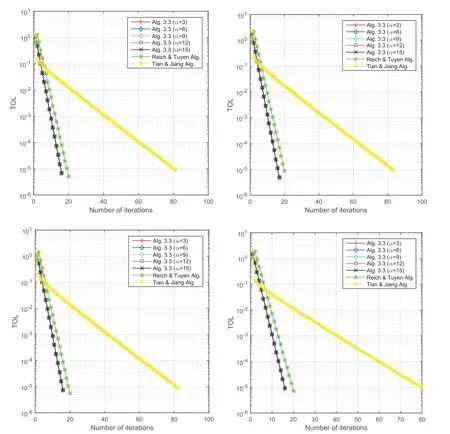
Figure 3 The behavior of TOLn with ε=10-5 for Example 5.3:Top Left: Case 1;Top Right: Case 2;Bottom Left: Case 3;Bottom Right: Case 4

Furthermore,the following were observed from our numerical experiments:

· We have seen from the numerical examples that the projections onto feasible sets are generally difficult to compute.Thus,the benefits brought from the half-space technique (introduced in our methods) are further verified by our numerical experiments.

· In the numerical experiments,we choose the parametersη≥0,λ1＞0 andμ1＞0 randomly and observed that the number of iteration does not change and no significant difference in the CPU time irrespective of the choices of the parameters.

· In each of the examples,we check the sensitivity ofαas we varyφ(φn) for each starting points,in order to know if these choices affect the efficiency of our methods.We can see from the tables and graphs that the gap between the best results and the worst results of Algorithm 3.2 and Algorithm 3.3 is acceptably small,especially in Example 5.2 and Example 5.3.We can also see from Table 1 and Figure 1 that for solving problem (5.1),the efficiency of Algorithm 3.2 is slightly affected by the dimensionality of the problem.These means that the proposed relaxed inertial technique has efficient and stable performance for each group of random data.

· It can also be inferred from the tables and figures that in terms of both CPU time and number of iterations,our proposed Algorithm 3.2 outperforms the method of He et al.[20,Algorithm 1] in Example 5.1 and Example 5.2,while our proposed Algorithm 3.3 outperforms the methods of Reich and Tuyen [47,Theorem 4.4] and Tian and Jiang [55,Algorithm (4.8)] in Example 5.3.Hence,our methods are more efficient and more implementable than these other methods for solving the SVIP.

6 Conclusion

In this paper,we studied two relaxed inertial methods which were developed from an explicit discretization of a dynamical system in real Hilbert spaces.Using these methods,we solved the SVIP (1.1)–(1.2) when the underlying operators are monotone and Lipschitz continuous.The Lipschitz constants of the underlying operators are known in the first proposed method while they are unknown in the second method.The main advantages of our proposed methods are that they do not require the SVIP (1.1)–(1.2) to be transformed into an equivalent VIP in a product space (hence,they utilize the attractive splitting structure of the SVIP);they are more implementable than other methods in the literature for solving the SVIP since they require only two projections onto half spaces per iteration with no further projection onto feasible sets;they involve inertial and relaxation steps which increases the convergence speed;and most importantly,our methods require the underlying operators to be freed from the usual and restrictive co-coerciveness assumption.Moreover,our analysis shows that the proposed methods converge strongly to a minimum-norm solution of the problem without relying on the usual “Two Cases Approach” which have been used to guarantee strong convergence in many papers.A direct consequence of our results is that our methods can be reduced to the RITFBF (1.7) for solving the classical VIP,when the projection is onto a half-space only,and the underlying operator is monotone and Lipschitz continuous,for which the Lipschitz constant may be known or unknown.Furthermore,we carried out some numerical experiments on our proposed methods and compared them with other methods for solving the SVIP.The results from the experiments shows that our methods are easily implemented and they also perform better than these other methods in literature.However,the proposed methods involve two evaluations ofAandFat each iteration which may affect the efficiency of the methods,especially in situations where the computations of the operators are expensive (for instance,in huge-scale problems).One of our future projects is to modify Algorithm 3.2 and Algorithm 3.3 in order to have only one evaluation ofAandFat each iteration

Appendix 6.1Algorithm 1 of He et al.[20].

Stop 0Given a symmetric positive definite matrix H ∈Rm×m,γ∈(0,2) andρ∈(ρmin,3),whereandT: RN→Rmis a linear operator (whereTTmeans the transpose ofT).Set an initial pointu1:=(x1,y1,λ1) ∈Ω :=C ×Q×Rm,where C and Q are nonempty closed and convex subsets of RNand Rm,respectively.

Step 1Generate a predictorwith appropriate parametersμ1andμ2:

Step 2Update the next iterativeun+1:=(xn+1,yn+1,λn+1) via

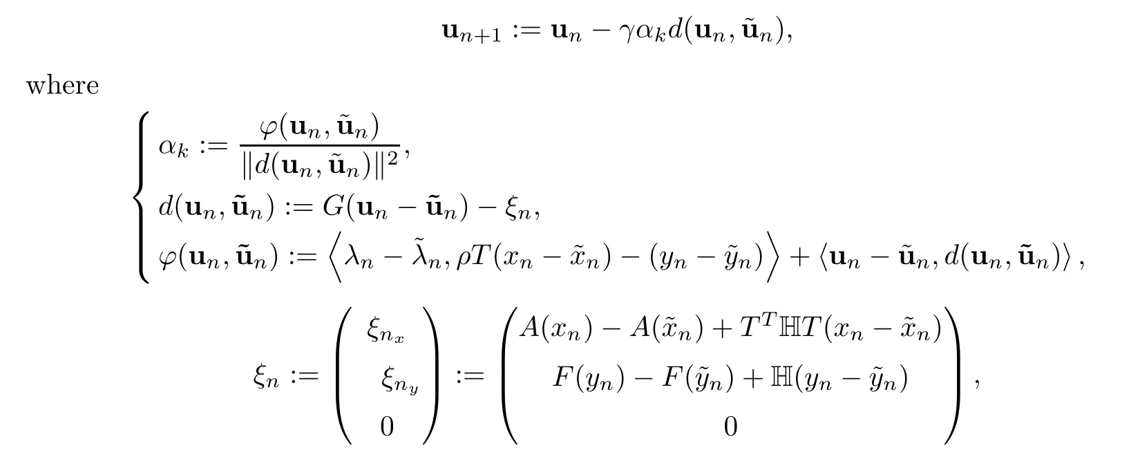
AandFare monotone and Lipschitz continuous with constantsL1andL2respectively,and

is the block diagonal matrix,with identity matricesINandImof sizeNandm,respectively.

The parametersμ1andμ2are chosen such that

wherev∈(0,1).

Appendix 6.2The Algorithm in Reich and Tuyen [47,Theorem 4.4].

For any initial guessx1=x∈H1,define the sequence {xn} by

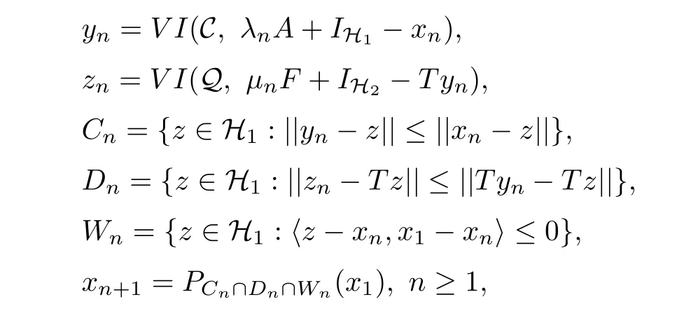
whereIH1andIH2are identity operators in H1and H2respectively,and {λn} and {μn} are two given sequences of positive numbers satisfying the following condition:

Appendix 6.3Algorithm (4.8) of Tian and Jiang [55].

Let {xn},{yn},{tn} and {wn} be sequences generated byx1=x∈C and

whereT: H1→H2is a bounded linear operator,A: C →H1is a monotone andL-Lipschitz continuous operator withL ＞0,F: H2→H2is ak-inverse strongly monotone mapping andh: H1→H1is aσ-contractive mapping with 0 ≤σ ＜1.The sequence {ηn} is in [a,b],for somea,b∈,{λn} is in [c,d],for somec,d∈,{αn} is in (0,1) withand