Hiroshi Sakai ?, Michinori Nakata

1Graduate School of Engineering, Kyushu Institute of Technology, Sensui 1-1, Tobata, Kitakyushu 804-8550, Japan

2Faculty of Management and Information Science, Josai International University, Gumyo, Togane, Chiba 283-0002, Japan

Abstract: The authors have been coping with new computational methodologies such as rough sets, information incompleteness, data mining, granular computing, etc., and developed some software tools on association rules as well as new mathematical frameworks. They simply term this research Rough sets Non-deterministic Information Analysis (RNIA). They followed several novel types of research, especially Pawlak’s rough sets, Lipski’s incomplete information databases, Or?owska’s non-deterministic information systems, Agrawal’s Apriori algorithm. These are outstanding researches related to information incompleteness, data mining, and rule generation. They have been trying to combine such novel researches, and they have been trying to realise more intelligent rule generator handling data sets with information incompleteness. This study surveys the authors’ research highlights on rule generators, and considers a combination of them.

1 Introduction

This paper focuses on some algorithms for rule generation from table data sets with uncertainty, and surveys our research highlights on rule generators. We also consider the perspective toward a more intelligent rule generation. The key concepts in this paper are rough sets [1–3], incomplete information databases [4, 5], nondeterministic information systems (NISs) [2, 6], and the Apriori algorithm [7–9]. Each research is outstanding, and we merge them for handling more intelligent rule generator.

The concept of rough sets proposed by Pawlak offers us a mathematical framework for analysing table data sets. A pair [A,v]of an attribute A and its attribute value v has termed a descriptor.Each descriptor [A,v] defines an equivalence class over the total set of objects (or instances). We can make use of equivalence classes for knowing the consistency and data dependency[3,10,11].

Incomplete information databases[4,5]and NISs[2,6]are similar frameworks for handling information incompleteness in table data sets. They employ a set P of possible values for dealing with information incompleteness, and interpret this set as that ‘a(chǎn) value in P is the actual value, but we do not decide it’ [2, 6]. For example,let us suppose Jack is an undergraduate student in Japan. In this case, even if we do not know Jack’s precise age, we will estimate that his age is between 18 years old and maximally 25 years old,namely non-deterministic information P={18,19,20,21,22,23,24,25}. Lipski coped with such non-deterministic information, and developed modal question-answering based on possible world semantics [4, 5, 12]. He clarified the sound and complete query translation axioms,which is known as S4,for query processing.

Both rough sets and incomplete information databases are related to table data sets, and it seems natural to consider rough sets for tables with information incompleteness. There seem several types of research coping with this issue, however, most of them seem to investigate the property of rough sets and not connected with the implementation of the actual system directly. There seems a gap between the model of rough set-based rule generation and the implementation of the rule generator. Furthermore, even in a standard table, the problem to obtain all minimal reducts is proved to be NP-hard [11]. Therefore, the logical property of completeness may often be ignored (this means there may be another rule except for the obtained rules). If we handle NISs according to the way of possible world semantics, generally the amount of the possible worlds increases exponentially. In the Congressional Voting data sets [13], the amount of possible worlds exceeds more than 10100. It seems hard to examine all possible worlds sequentially. (Actually, in the subsequent sections we gave a solution to this problem, and propose rule generation according to the way of possible world semantics.) We have to pay attention to the computational complexity on rule generation as well as rough set-based rule generation model.

The Apriori algorithm proposed by Agrawal et al.[7–9]is known as a novel approach to data mining and knowledge discovery[7,8],which has led various data mining studies.This algorithm originally handled data in transaction form, but it can consider the Apriori algorithm for table data sets by looking at a descriptor as one item[14]. We term this algorithm the Deterministic Information System(DIS)-Apriori algorithm (Apriori algorithm for DISs), and extend it to the NIS-Apriori algorithm (Apriori algorithm for NISs). These algorithms preserve logical properties soundness and completeness for a set of rules [15].

To examine the validity of the proposed algorithms, crossvalidation evaluation is often employed [16]. However, we do not employ cross-validation evaluation, because to prove the logical properties soundness and completeness is another way to validate the proposed algorithms. The proposed algorithm detects each implication τ if and only if τ is satisfying the condition of a rule.These properties theoretically assure the validity of algorithms.This is an advantage of the logic-based framework.

In this paper,we clarify the above researches by using an example data set, and investigate the role and the property of them. More concretely, we sequentially focus on the following:

(1) Rough set-based consistent rule generation

(1A) Rule generation by the definability of a set in DISs,

(1B) Rule generation by the definability of a set in NISs,

(1C) Rule generation by the discernibility function in NISs.

(2) Apriori-based rule generation,

(2A) DIS-Apriori-based rule generation from DISs,

(2B) NIS-Apriori-based rule generation from NISs,

(2C) Rule generation by the NIS-Apriori with a target descriptor.

This paper is organised as follows.Section 2 considers(1A),and Section 3 copes with (1B). Section 4 reviews the discernibility function and considers (1C). Section 5 copes with (2A), and Section 6 does (2B). In each section, we present the actual execution logs. Section 7 compares two types of rule generation,and clarifies the advantage and disadvantage of each rule generation. Then, we combine two types of rule generation, and propose (2C). Section 8 concludes this paper.

2 Rough set-based consistent rule generation in DISs

A DIS ψ is a quadruplet

where OB is a finite set whose elements are called objects or instances, AT is a finite set whose elements are called attributes,VALAis a finite set whose elements are called attribute values of A ∈AT, and f is such a mapping [1, 3, 11]

We say objects x and y are indiscernible for ATR,if f(x,A)=f(y,A)for every A ∈ATR ?AT. In rough sets, the following indiscernibility relation for ATR is employed. This relation is also an equivalence relation over OB.

where the term [x]ATRand eq(ATR) an equivalence class with an object x and a set of all equivalence classes for ATR, respectively.If a set X ?OB satisfies the equation X =∪x∈OB[x]ATR, we say X is definable in DIS. (Actually, there is a subset OB′?OB and it is enough to consider OB′.) If X is definable in DIS, it can characterise the set X by using the condition ∧A∈ATR[A,f(x,A)](x ∈X).If X is not definable,X is approximated by the next two sets

Generally,a pair(Lower App,UpperApp)is termed rough sets of X.We approximate the set X by LowerApp and UpperApp which are both definable. The details are in [1, 3, 11].

Let CON ?AT and Dec ∈AT denote the condition attributes and a decision attribute,respectively.An object x ∈OB is consistent with other y ∈OB for CON and Dec, if f(y,A)=f(x,A) for every A ∈CON implies f(y,Dec)=f(x,Dec). If x ∈OB is consistent,we say ∧A∈CON[A,f(x,A)]?[Dec,f(x,Dec)] is a consistent implication. Here, we focus on an important proposition, which clarifies the concept of consistency and equivalence classes.

Proposition 1: In DISs, the following two conditions are equivalent [3]:

(i) An object x ∈OB is consistent with other y ∈OB for CON and Dec.

(ii) [x]CON?[x]Dec.

Proposition 1 connects the concept of consistent implications with the inclusion relation between equivalence classes. At the beginning of Pawlak’s work, a rule was dealt with as a consistent implication, and the inclusion relation was examined for consistent rule generation. Let us show each concept by using an example.

Example 1: We employ DIS ψ1in Table 1, and clarify each definition.

(i)In ψ1,eq({A})={{1,3},{2,4}}holds.A set OB={1,2,3,4}is definable,because OB={1,3}∪{2,4}for an attribute set{A},but a set X ={1,2,3} is not definable. In this case, rough sets({1, 3}, {1, 2, 3, 4}) approximate the set X. For an attribute set{A,B}, eq({A,B})={{1,3},{2},{4}} holds. In this case, X is definable, and rough sets of X is ({1, 2, 3}, {1, 2, 3}).(ii) To specify conditions in tables, we employ a descriptor like[Dec,2] (it means Dec=2). The descriptor [Dec,2] specifies a set X′={2,3}, and we consider the definability of X′={2,3}.In eq({A}), X′is not definable, and rough sets are (?,{1,2,3,4}).In eq({A,B}),X′is not definable,and rough sets are({2},{1,2,3}).(iii) In eq({A}), equivalence classes {1, 3} and {2, 4} are specified by [A,2] and [A,1], respectively. Therefore, the set OB is characterised by the condition [A,1]∨[A,2], and we have an implication[A,1]∨[A,2]?[Dec,1]∨[Dec,2]∨[Dec,3]. In eq({A,B}),{2}?X′holds. This means {2} is a lower approximation of X′.So, a consistent implication is obtained from object 2 by using Proposition 1, and we have [A,1]∧[B,2]?[Dec,2].

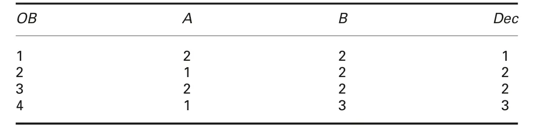
Table 1 Exemplary DIS ψ1

In Example 1,a property among rules,definability of a set,and lower approximation are shown.Because the conjunction ∧A∈ATR[A,valA]of descriptors defines an equivalence class [x]∧A∈ATR[A,valA], we have a consistent implication ∧A∈ATR[A,valA]?[Dec,val], if we find an inclusion relation [x]∧A∈ATR[A,valA]?X (X is specified by [Dec,val]). Pawlak’s framework is extended to variable precision rough sets (VPRSs) [17] and other several research areas[10, 11, 16, 18–30].

3 Consistent rule generation in NISs

3.1 Rules in NISs and possible equivalence relations

A NIS Φ is also a quadruplet [2, 6]

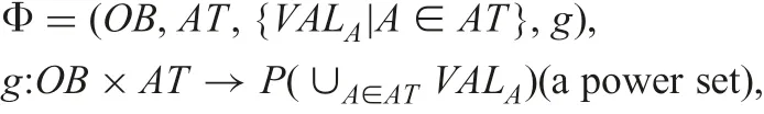
where g is a mapping from OB×AT to a power set of ∪A∈ATVALA.The interpretation of each set g(x,A) characterises the meaning of NIS. We interpret it as that an actual value is in g(x,A), but we cannot specify the actual value without additional information. The set g(x,A)is equal to VALA,if we do not have any information of x.

NIS was investigated by Or?owska and Pawlak, and information incompleteness in table data sets was discussed. The framework of incomplete information databases [4, 5] was also proposed by Lipski for handling question-answering under uncertain information. Relational algebra and null values by Codd [31] were followed by these researches.

In about 1985,new research areas like data mining and knowledge discovery emerged in addition to IR and question-answering in databases, and the problem on NISs also seemed to be transferred to the problem on missing values. The framework of learning from examples with unknown attribute values [32] was proposed. Rules from tables with missing values were investigated [21]. However,some assumptions are required in such research on missing values,and the interpretation of such assumptions seems complicated and vague. For this reason, we follow the original definition of NISs instead of considering missing values with some assumptions. Our framework and the framework handling missing values are different,and the obtainable rules in NISs are slightly different from the rules with an assumption of missing values [14].

Definition 1: For NIS Φ= (OB,AT,{VALA|A ∈AT},g), we fix a set ATR ?AT and such a mapping h:OB×ATR →∪A∈ATRVALAthat h(x,A)∈g(x,A). We term DIS ψ= (OB,ATR,{VALA|A ∈AT},h) a derived DIS from NIS Φ [33].

Definition 2:Let DD(Φ)denote a set{ψ|ψ is a derived DIS from Φ}.We also term equivalence classes in a derived DIS ψ a possible equivalence class (pe-class) in Φ. Let peq(ATR,ψ) be a set of all pe-classes in ψ ∈DD(Φ) [33].

Example 2:A table Φ1in Table 2 is an exemplary NIS.In Φ1,there are 48 (=24×3) derived DISs for ATR={A,B,Dec}. Table 3 shows a derived DIS ψ from Φ1. In this derived DIS ψ,eq({A,B})={{1},{2},{3},{4},{5},{6,7},{8}}, and this is peq({A,B},ψ). Each element in peq({A,B},ψ) is a pe-class in Φ1. There are 48 derived DISs for Φ1, so there may exist 48 different peq({A,B},ψ).

Remark 1:

(i)In Section 2,we examined the relation between rules in DISs and equivalence relations. Thus in NISs, it is necessary to consider the relation between rules in NISs and pe-classes.

(ii) In NIS Φ, we see that there is an actual derived DIS ψactual∈DD(Φ) based on the definition of non-deterministic information. In NIS Φ, we characterise rules which certainly hold in ψactualand rules which possibly hold in ψactual. Definitions 1, 2,ψactual, certainty, and possibility follow the idea of Lipski’s incomplete information databases [4, 5].

(iii)In rough sets with respect to DISs,the purpose is to characterise the set X specified by a descriptor[Dec,val],however,in NISs,we characterise implications based on ψactual. Both frameworks are related to rule generation, but the character of the obtained rules is different.

Definition 3: (A simplified definition) [33]:

(i)An implication τ:∧A∈CON[A,valA]?[Dec,val]is a certain and consistent rule(c-c rule),if τ is a consistent rule in each ψ ∈DD(Φ).(ii) An implication τ:∧A∈CON[A,valA]?[Dec,val] is a possible and consistent rule (p-c rule), if τ is a consistent rule in at least one ψ ∈DD(Φ).Clearly, one c-c rule becomes a p-c rule. If each g(x,A) in Φ is a singleton set, we identify this Φ with one DIS ψ, and DD(Φ)={ψ} holds. Therefore, (1) and (2) in Definition 3 define the same implications, and Definition 3 covers the rules in not only NIS but also DIS. We see that Definition 3 is a natural extension of consistent rules in DISs.We have the following remark.

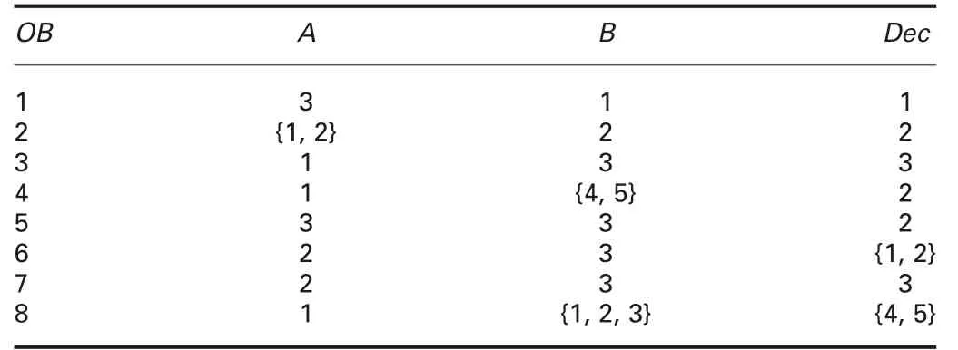
Table 2 Exemplary NIS Φ1

Table 3 Derived DIS ψ from Φ1

Remark 2:

(i) If an implication τ:∧A∈CON[A,valA]?[Dec,val] is a c-c rule,this τ is a consistent rule in the unknown actual ψactual.

(ii)If an implication τ:∧A∈CON[A,valA]?[Dec,val]is a p-c rule,this τ may be a consistent rule in the unknown actual ψactual.

(iii) If an implication τ:∧A∈CON[A,valA]?[Dec,val] is not a p-c rule, this τ is not any rule in the unknown actual ψactual.

(iv) Rule generation in NISs considers the certainty and the possibility of rules for the unknown actual DIS ψactual.

3.2 Consistent rule generation by the definability of a set in NISs and manipulation of pe-classes in Prolog

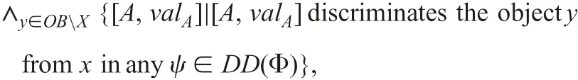
Let us consider the definability of a set X specified by a descriptor[Dec,val]. In DIS ψ, the equivalence relation eq(ATR) is unique, but in NISs there are plural peq(ATR,ψ) (ψ ∈DD(Φ)).Algorithm 1 (see Fig. 1) employs the backtrack procedure, and examines the definability of a set X.

Let’s consider Example 1,again.If we select CON ={A,B},we have eq({A,B})={{1,3},{2},{4}}. For X ={1,2,3,4}=OB,Algorithm 1 (Fig. 1) fixes X?={1,2,3,4}, picks up [1]{A,B}={1,3}, and assigns X?={1,2,3,4}{1,3}={2,4}. Then,X?={2,4}{2} are generated, and X?={4}{4}=? is derived. Thus, we know OB is definable. (In reality, OB has been always defined.)

Algorithm 1(Fig.1)is related to the algorithm LEM[32].The set CL is unique in every DIS,because CL is an equivalence class with an object x.However,the set CL in NIS is a pe-class,so it may not be unique.Thus,search with backtrack is necessary for finding all CL.Algorithm 1 (Fig. 1) is different from the LEM algorithm at this point.

As for the definability of a set, we can define certainly definable and possibly definable like Definition 3. In this definition, a new concept of the definability of a set is investigated. By extending Algorithm 1 (Fig. 1), we implemented a software tool handling two concepts, certainly definable and possibly definable. In the following,we explain them through the actual execution on NIS Φ1.

Fig. 1 Algorithm 1: (Definability of a set in NISs) [33]

It is generally difficult to simulate the backtrack functionality by using the procedural programming language, so we employed Prolog, because Prolog is originally equipped with the backtrack functionality. Every program handling pe-classes and data dependency is implemented in Prolog on Windows PC (Core i7 CPU,3.6 GHz). We at first prepare the following data set caai.pl in Prolog, whose contents are in Table 2.

object(8,3).

data(1,[3,1,1]), data(2,[[1,2],2,2]),

data(3,[1,3,3]), data(4,[1,[4,5],2]),

data(5,[3,3,2]), data(6,[2,3,[1,2]]),

data(7,[2,3,3]). data(8,[1,[1,2,3],[4,5]]).

We employ a file attrib.pl for defining the attributes,whose contents are decision([3]) and condition([1,2]). The content decision([3]) specifies the decision attribute (third attribute), i.e. Dec, and condition([1,2]) does the first (A)and the second (B) is condition attributes. Since OB is definable by any peq(ATR,ψ), we can obtain any set of pe-classes by examining the definability of OB. Fig. 2 shows this.

In Fig.3,the definability of sets{1,4,5}and{3,4}is examined.As a side effect of Algorithm 1 (Fig. 1), some pe-classes are obtained. The set {1, 4, 5} is definable in each of 48 derived DISs. In the execution, Remark 2 is internally applied to the definability of a set.

In Fig.4,information on data dependency is displayed.There are 48 derived DISs from Φ1, and there exists no consistent DIS. The maximum degree of dependency from {A,B} to Dec is 0.75 in 48 derived DISs, and the minimum degree is 0.5. Thus, the degree of dependency in ψactualis between 0.5 and 0.75. Objects 1, 4, and 5 are consistent in each of 48 derived DISs. This was also shown that a set {1, 4, 5} is definable in each of 48 derived DISs in Fig. 3. Based on Figs. 3 and 4, we know that it is possible to generate c-c rules below:

If we employ one disjunction ∨, it is possible to generate c-c rule([B,4]∨[B,5])?[Dec,2] from object 4.

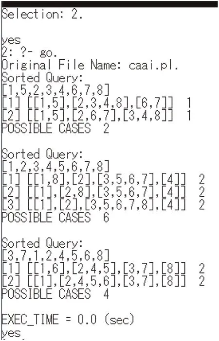
Fig. 2 Sets of all pe-classes in each attribute are displayed. For example,peq({A},ψ)={{1,5},{2,3,4,8},{6,7}} occurs one time on the attribute A, and it consists of three pe-classes. Similarly,peq({B},ψ)={{1},{2},{3,5,6,7,8},{4}} occurs two times for the attribute B, and peq({Dec},ψ)={{1},{2,4,5,6},{3,7},{8}} occurs two times for the attribute Dec

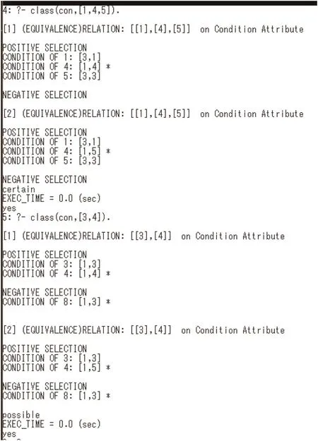
Fig. 3 Definability of two sets {1, 4, 5} and {3, 4}. The set {1, 4, 5} is examined as certainly definable in Φ1. The term ‘certain’ over the execution time implies that the set is certainly definable. The set {3, 4} is possibly definable. This execution is based on Remark 2

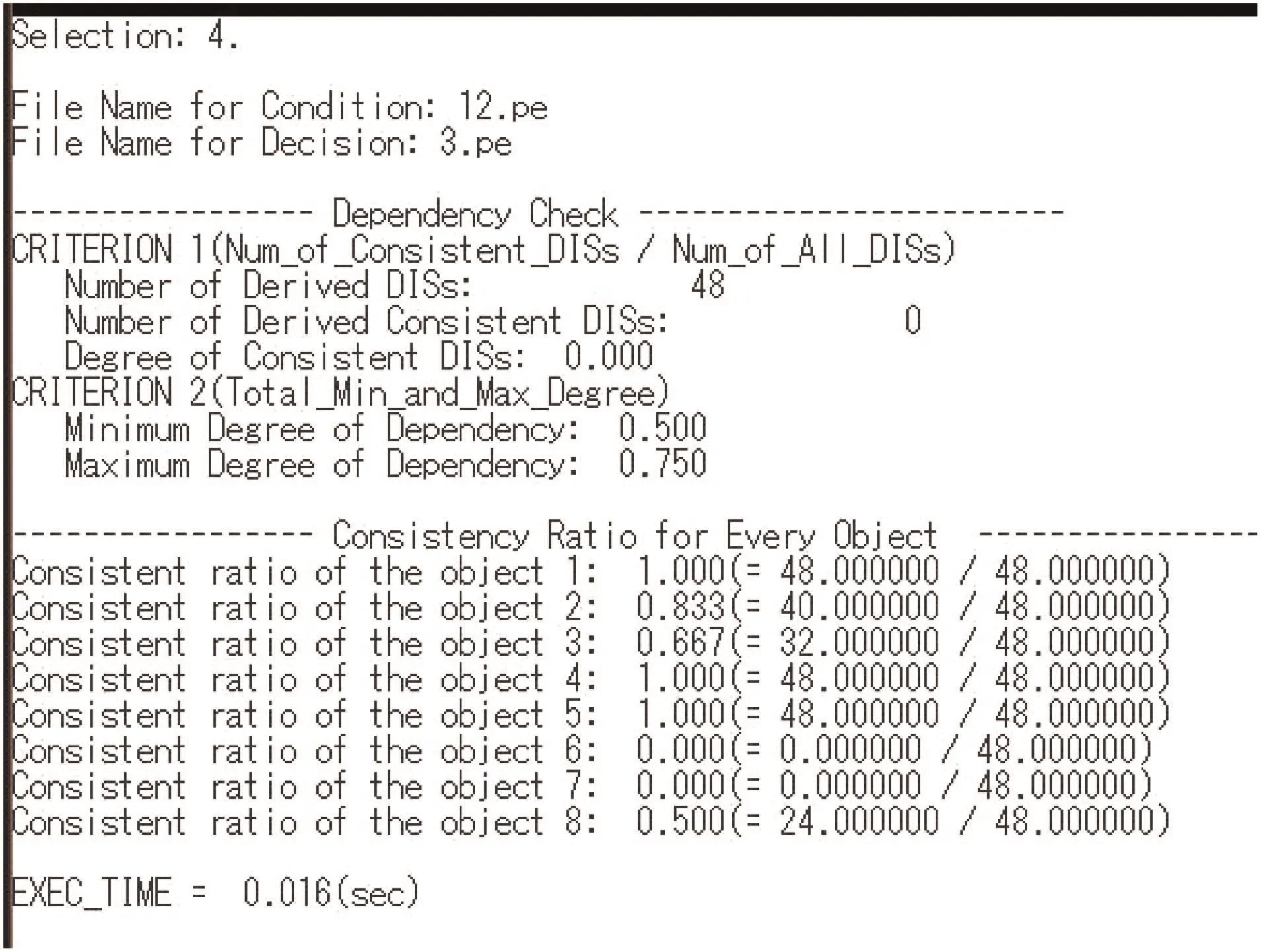
Fig. 4 Information on data dependency from {A,B} to Dec

We have briefly described a set of pe-classes defined by NISs and its manipulation in Prolog powered by Algorithm 1(Fig.1).A more detailed explanation is in [33–35]. Actually, Algorithm 1 (Fig. 1)employs exhaustive search over pe-classes, so the complexity of calculation depends upon the amount of |DD(Φ)|. Generally,|DD(Φ)| increases exponentially. Even in Φ1, the amount of|DD(Φ1)| is 48. Thus, Algorithm 1 (Fig. 1) will not be suitable to generate rules from large size data sets. The application of the pe-manipulation system in Prolog will be restricted to small size data sets.

4 Consistent rule generation by the discernibility function method

In rough sets, we can easily obtain a consistent rule by finding one lower approximation of X specified by a decision [Dec,val].However, a generally lower approximation may not be unique,so it is necessary to find all lower approximations to obtain all consistent implications. Skowron proposed the discernibility function, and the problem to determine all minimal reducts was translated to an SAT problem (to obtain solutions of the conjunctions of disjunction of descriptors). Thus, Skowron proved that ‘to determine all minimal reducts is NP-hard’ [11], so it is not easy to enumerate all lower approximations for large data sets.However, the discernibility function method (df-method) affords a way to enumerate each lower approximations. If each solution of the discernibility function is examined, the df-method preserves the logical property on rule generation below:

Soundness) The df-method generates only consistent implications.Completeness) Any consistent implication is obtainable by the df-method.

Generally,the property of soundness will be equipped with every system, and the property of completeness assures that no rule is missed in rule generation. So, completeness will be a preferred property. However it sometimes seems to be ignored in rough set-based systems due to the Skowron’s result of NP-hard.

Example 3:(1)Let’s consider Example 1 and the decision[Dec,3].Since[Dec,3]specifies X ={4},therefore,we discriminate objects 1,2,and 3 by using A and B.As for object 1,both[A,1]and[B,3]discriminate object 1 from object 4. As for object 2, [B,3] does object 2 from object 4, and [A,1] and [B,3] discriminate object 3 from object 4. Thus, we have a discernibility function df(4)=([A,1]∨[B,3])∧[B,3]∧([A,1]∨[B,3]). The solution to df(4)becomes the condition part of consistent rules. The minimum solution is [B,3], and we have a minimum consistent rule[B,3]?[Dec,3].

We have extended the df-method in DISs to the df-method in NISs[36]. In the df-method in NISs, a set X of objects must be discriminated from any object in OBX in each of derived DISs. For handling this, a new discernibility function was defined[36]. Fig. 5 is a log data for generating c-c rules from Φ1in Table 2. This software tool is also implemented in Prolog. By using Fig. 5, we explain the overview of the df-method in NISs sequentially.

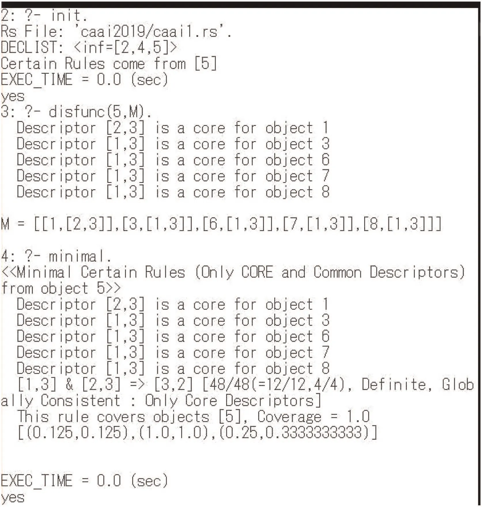
Fig. 5 Log data for c-c rule generation from Φ1

(i)At first,we define a descriptor[Dec,2]as the decision part,and it is stored in the attrib.pl file. The data set caai.pl is translated to caai1.rs file by using the attrib.pl file. In this caai1.rs, information on pe-classes are stored.

(ii) The init command examines each object whose decision part is[Dec,2],and inf=[2,4,5]is displayed.For each object 2,4,and 5, the definability of an object is examined, and only object 5 is detected as certainly definable. Thus, c-c rules can be obtainable from object 5.

(iii) Since c-c rule in Definition 3 is a consistent rule in each of derived DISs, the discernibility function in Φ1needs to discriminate objects 1, 3, 6, 7, 8 from object 5 in each of 48 derived DISs. Here, [8, 18] (it means [B,3]) discriminates object 1 from object 5, [7, 18] (it means [A,3]) does objects 3, 6, 7, and 8.In this case, the authors of [8, 18] can discriminate object 8 in some derived DISs but not 48 derived DISs. Thus, the authors [8,18] cannot be employed for discriminating object 8. This is the extended part of the discernibility function in NISs.

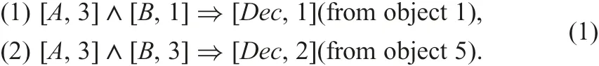
(iv) The discernibility function df(5) is displayed in Fig. 5. In this case, the solution of df(5) is uniquely [1,3]∧[2,3], and we have a minimum c-c rule [A,3]∧[B,3]?[Dec,2] from object 5,which is shown in formula (1).

(v) To obtain all c-c rules, we need to change the decision part[Dec,2] to [Dec,1], [Dec,3], [Dec,4], [Dec,5], and need to repeat the same steps for each decision part.

We briefly described the df-method in NISs by using an actual execution log. The next discernibility function

affords an intuitive way to enumerate each lower approximation.However, for large size data sets, to have all solutions of df(x)becomes a satisfiability problem, SAT. Therefore, the df-method will not be suitable for generating rules from large size data sets.The application of the df-method in Prolog will also be restricted to small size data sets. It is necessary to employ an exhaustive search for finding all lower approximations. We have implemented some variations of a software tool to obtain lower approximations.In one of them, we can sequentially specify some descriptors for reducing the size of df(x) [35, 36].

5 Apriori-based rule generation

We focus on the Apriori algorithm,and extend it to the NIS-Apriori algorithm and NIS-Apriori in SQL.

5.1 Apriori algorithm and rules in DISs

The Apriori algorithm was originally defined for handling the transaction format data, and the operation of item sets was investigated [7]. The Apriori algorithm is known as one of the famous algorithms for knowledge discovery [9]. Generally, the decision part is not fixed in the Apriori algorithm, and the purpose is to obtain association rules defined by each frequent item set.

However, if we recognise an item with a descriptor [A,valA] in table data sets, it is possible to apply the Apriori algorithm to rule generation from table data sets. In DIS ψ1in Table 1, we see each tuple shows an item set,and the table ψ1is a set of item sets below:

ItemSet(1)={[A,2],[B,2],[Dec,1]},

: : :

ItemSet(4)={[A,1],[B,3],[Dec,3]},

Tuple(ψ1)={ItemSet(1),ItemSet(2), ...,ItemSet(4)}.

We termed the algorithm handling the above data structure a DIS-Apriori algorithm. The relation between the Apriori algorithm and the DIS-Apriori algorithm is below:

(1) The amount of elements in each ItemSet(i) is the same as the number of attributes.

(2)The decision attribute Dec is usually predefined,and the decision part is an element in the set {[Dec,val]|val ∈VALDec}.

(3)Except (1)and(2),the DIS-Apriori algorithm is almost equal to the Apriori algorithm.

In rough sets, rules are originally identified with a consistent implication, and we described methods to obtain consistent implications in the previous sections. However, the consistency on implications is often too strict, so the definition of rules was extended to VPRS [17]. Similarly, in the Apriori algorithm,the criterion values support and accuracy (or confidence) are employed. We follow the research on rules, and we consider the next definition.

Definition 4:For DIS ψ,two given threshold values 0 ＜α,β ≤1.0,an implication τ:∧A∈CON[A,valA]?[Dec,val] satisfying (1) and(2) is called (a candidate of) a rule in ψ [3, 7, 11, 37].

Here eq(?) is an equivalence class defined by the formula ?. If|eq(∧A∈CON[A,valA])|=0, we define both support(τ)=0 and accuracy(τ)=0.

Remark 3:

(i) The consistent implications, which are dealt with as rules in the previous sections, corresponding to the case of accuracy(τ)=1.0 in Definition 4. Therefore, Definition 4 extends the concept of consistent rules.

(ii) Rough set-based rule generation employs Proposition 1 and selects accuracy(τ) as a top priority for rule generation. The selection of lower approximations means to generate rules satisfying accuracy(τ)=1.0.

(iii)Since both the pe-classes manipulation and the df-method handle only consistent implications, we cannot apply them to generating rules satisfying β ≤accuracy(τ)＜1.0. We need other methods handling rules in Definition 4.

5.2 DIS-Apriori algorithm and its simulation

This subsection clarifies the properties of the criterion values support(τ) and accuracy(τ) in rule generation. The next sets IMP1,IMP2, …, IMPnare also introduced.

IMP1={[A,valA]?[Dec,val]},(All implications with one condition attribute),

IMP2={[A,valA]∧[B,valB]?[Dec,val]},(All implications with two condition attributes),

IMP3={[A,valA]∧[B,valB]∧[C,valC]?[Dec,val]},(All implications with three condition attributes).

: : : :

Here, the subscript i in IMPiis the amount of descriptors in the condition part, and |IMPi| is the amount of implications. The purpose of Apriori-based rule generation is to detect implications in Definition 4 from ∪i=1,...,(|AT|-1)IMPi. Of course, we can examine each τ ∈∪i=1,...,(|AT|-1)IMPisequentially. However this trivial method will take much execution time. The Apriori algorithm employs the property on redundancy, and proposes a more effective method [7].

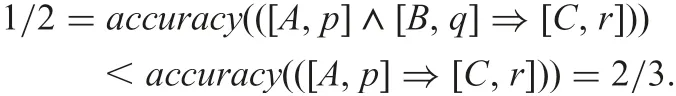
Definition 5: For an implication τ:∧A∈CON[A,valA]?[Dec,val]and any descriptor [B,valB] (B ?CON ∪{Dec}), we say τ′:((∧A∈CON[A,valA])∧[B,valB])?[Dec,val] is a redundant implication of τ [14, 15].

Definition 5 reduces the amount of rules, and we handle only minimal implications as rules.Since(P1∧P2?Q)=((P1?Q)∨(P2?Q)) holds, if we detect an implication P1?Q is a rule, we automatically see the redundant implication P1∧P2?Q is also a rule. (In this case, we ignore support(τ) condition, because support(τ) may be less than α for τ:P1∧P2?Q.)

Example 4: Now, we consider Table 4.

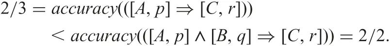
Namely, the accuracy value of the redundant implication is bigger.Then, we consider Table 5. In this case, the accuracy value of the redundant implication is lower.

Thus, we have the next properties on implication τ:[A,valA]?[Dec,val] and its redundant implication τ′[14, 15].

Property 1:If support(τ)＜α,any redundant implication τ′is not a rule, because support(τ′)≤support(τ) clearly holds.

Property 2: If support(τ)≥α and accuracy(τ)≥β, τ and any redundant τ′is a rule. (We only consider minimal implications as rules.)

Property 3: If support(τ)≥α and accuracy(τ)＜β, a redundant τ′may be a rule.

Base on three properties,we do not have to consider any redundant implication satisfying (Property 1) nor (Property 2). It is enough to consider any redundant implication satisfying (Property 3) for rule generation. Namely,we can consider the following set:

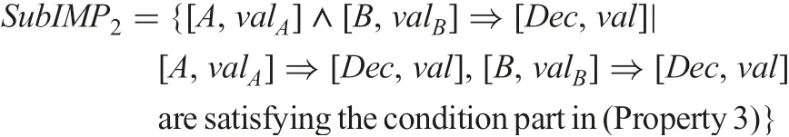
instead of IMP2.Generally,the amount of|SubIMP2|is much smaller than the amount of|IMP2|.

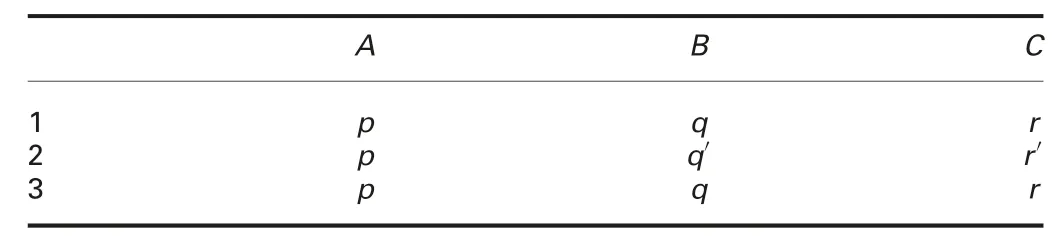
Table 4 Exemplary DIS ψ2

Table 5 Exemplary DIS ψ3

The DIS-Apriori algorithm in Algorithm 2(see Fig.6)makes use of SubIMPiand Properties 1–3. Since the DIS-Apriori algorithm handles ∪i=1,...,(|AT|-1)IMPiby using SubIMP2, SubIMP3, …, it is sound and complete for the rules in Definition 4. So, any rule specified in Definition 4 can be obtained by Algorithm 2 (Fig. 6).

Example 5: For ψ1in Table 1, let us fix α=0.1 and β=0.6.Then, each implication satisfies support(τ)≥0.1, and IMP1={τ1:[A,2]?[Dec,1],τ2:[A,1]?[Dec,2], τ3:[A,2]?[Dec,2],τ4:[A,1]?[Dec,3],τ5:[B,2]?[Dec,1],τ6:[B,2]?[Dec, 2],τ7:[B,3]?[Dec,3]}. Actually, Rule={τ6,τ7} and Rest ={τ1,τ2,τ3,τ4,τ5}, we need to consider four combinations, τ1and τ5, τ2and τ5, τ3and τ5, τ4and τ5, because [A,1]∧[A,2]is meaningless and [Dec,1]∧[Dec,3] is also meaningless.Only τ1and τ5is possible, so we have SubIMP2={τ8:[A,2]∧[B,2]?[Dec,1]}. Since accuracy(τ8)=0.5, τ8is not a rule.Thus, we have two minimal rules τ6:[B,2]?[Dec,2] and τ7:[B,3]?[Dec,3]. In Example 1, we obtained a consistent implication [A,1]∧[B,2]?[Dec,2], but τ6becomes a rule for accuracy(τ)≥0.6.

5.3 NIS-Apriori algorithm in NISs

We follow Definition 3,and consider the next rules in Definition 6.

Definition 6: We define the following [14, 37]:

(i) We say τ is a certain rule, if τ satisfies support(τ)≥α and accuracy(τ)≥β in each ψ ∈DD(Φ).

(ii) We say τ is a possible rule, if τ satisfies support(τ)≥α and accuracy(τ)≥β in at least one ψ ∈DD(Φ).

Remark 4: Similarly to Remark 2, we have to remark to the following.

(i) A certain rule τ is also a rule in ψactual, namely a certain rule characterises an implication τ which is certainly a rule in ψactual.

(ii)A possible rule τ may be a rule in ψactual,namely a possible rule characterises an implication τ which may be a rule in ψactual.

(iii) An implication, which is not a possible rule, characterises an implication τ which is definitely not a rule in ψactual.

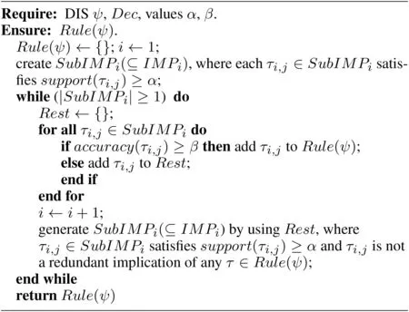
Fig. 6 Algorithm 2: (DIS-Apriori algorithm)

The rules in Definition 6 seem to be familiar in possible world semantics. However, the amount of elements in DD(Φ) increases exponentially, so we have the computational complexity problem for large size data sets. Even in Φ1, the amount is 48, and the amount is more than 10100in the Congressional Voting data set[13]. We defined the following two sets for a descriptor [A,val],which we make use of solving this computational problem.

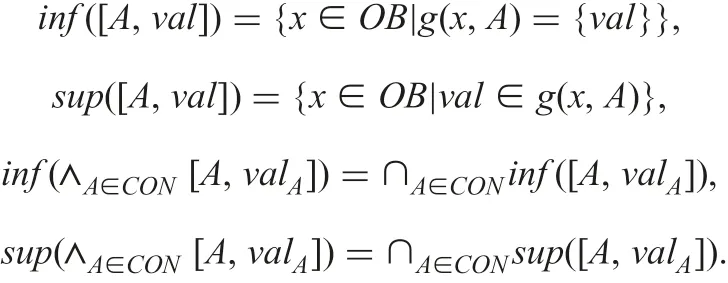
By making use of the sets inf and sup, we have solved the computational complexity problem below [14, 15].

(Result 1): There is a derived DIS ψmin∈DD(Φ) satisfying(i) and (ii).

(i) minsupp(τ)(=minψ∈DD(Φ){support(τ)in ψ})=support(τ) in ψmin.

(ii) minacc(τ)(=minψ∈DD(Φ){accuracy(τ)in ψ})=accuracy(τ) in ψmin.

(iii) Two criterion values are given as follows:

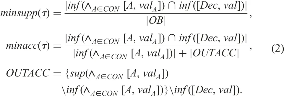
(Result 2): There is a derived DIS ψmax∈DD(Φ) satisfying(i) and (ii).

(i) maxsupp(τ)(=maxψ∈DD(Φ){support(τ)in ψ})=support(τ) in ψmax.

(ii) maxacc(τ)(=maxψ∈DD(Φ){accuracy(τ)in ψ})=accuracy(τ) in ψmax.

(iii) Two criterion values are given as follows:

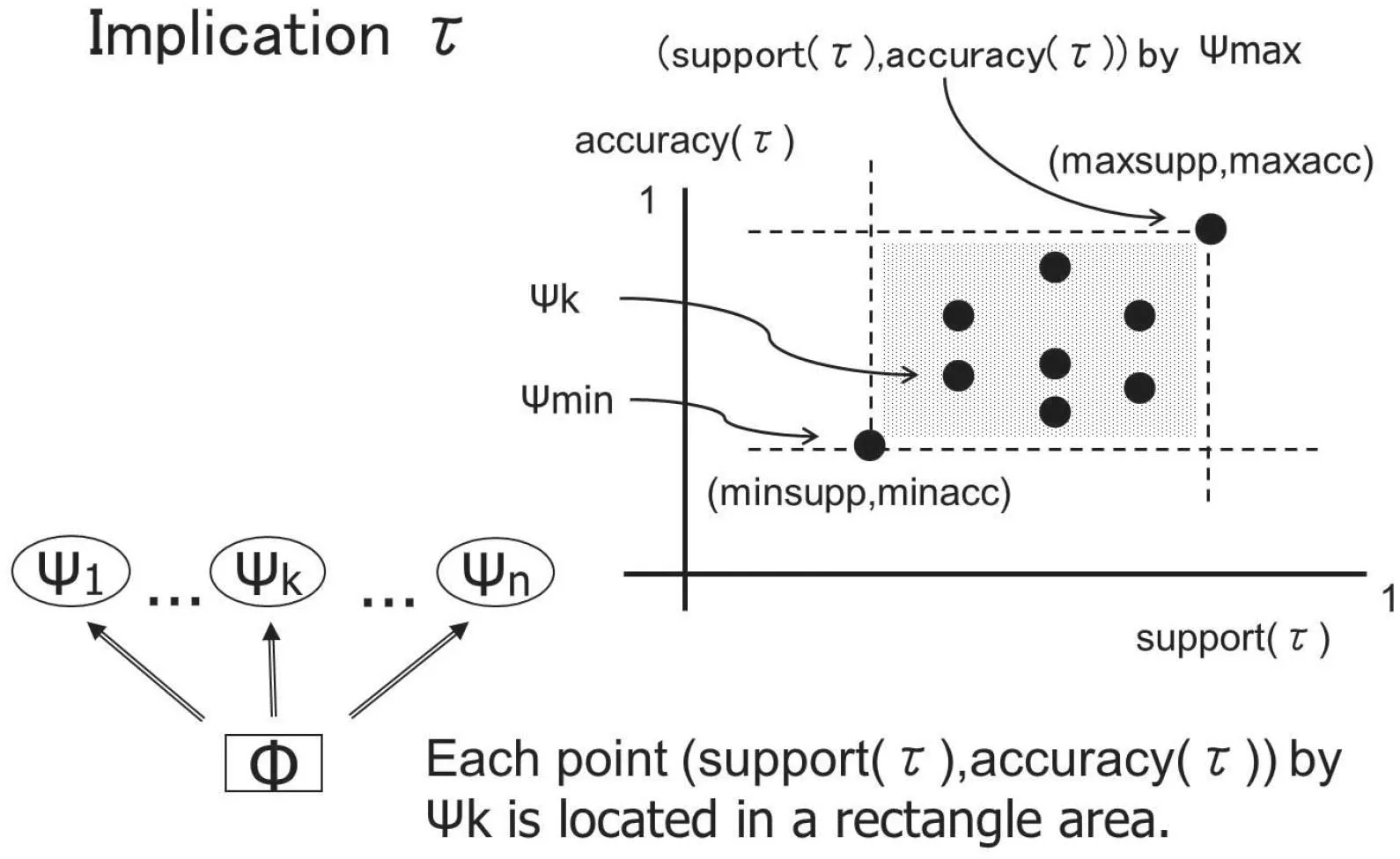
Fig. 7 Location of (support(τ),accuracy(τ)) by ψ ∈Φ [15]

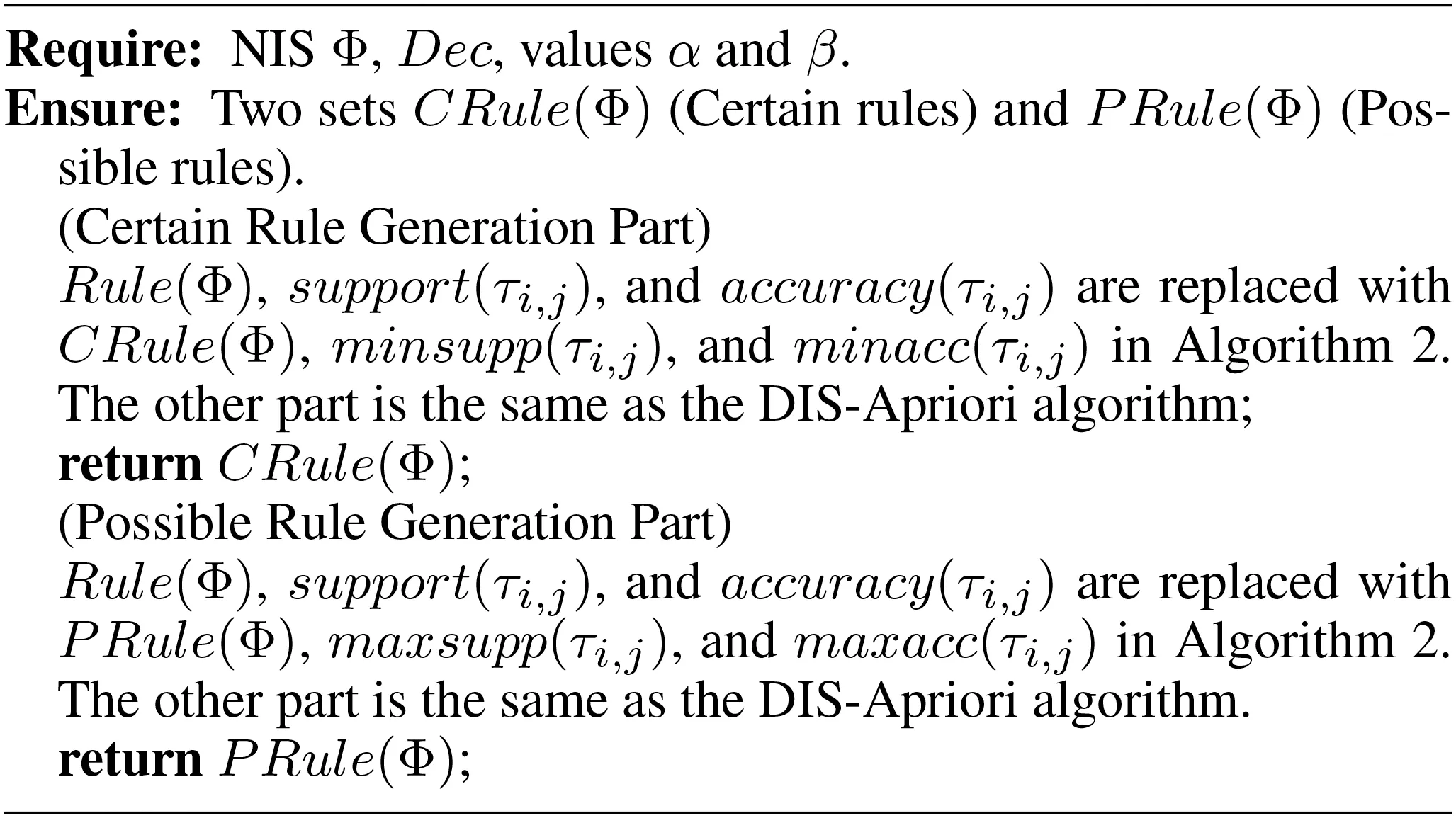
Fig. 8 Algorithm 3: (NIS-Apriori algorithm) [15]

(Result 3):Based on Results 1 and 2,we have Fig.7.Thus,τ is a certain rule, if and only if τ is a rule in ψmin∈DD(Φ), i.e.minsupp(τ)≥α and minacc(τ)≥β. An implication τ is a possible rule,if and only if τ is a rule in ψmax∈DD(Φ),i.e.maxsupp(τ)≥α and maxacc(τ)≥β. It is enough for us to consider ψminand ψmax,and we do not have to consider DD(Φ). Each formula of four criterion values, minsupp(τ), …, maxacc(τ), does not depend on the amount of DD(Φ). Thus, certain rule generation and possible rule generation do not depend upon the amount of elements in DD(Φ).

We apply the above three results to the DIS-Apriori algorithm in Algorithm 2 (Fig. 6), and we propose the NIS-Apriori algorithm in Algorithm 3 (see Fig. 8). Namely, in certain rule generation support(τ) and accuracy(τ) in Algorithm 2 (Fig. 6) are replaced with minsupp(τ)and minacc(τ),respectively.In a possible rule generation, maxsupp(τ) and maxacc(τ) are employed in Algorithm 2(Fig.6).Therefore,the time complexity of the NIS-Apriori algorithm is more than twice time complexities of the DIS-Apriori algorithm.However,we employ Results 1–3 and calculate four values in polynomial order time, thus the NIS-Apriori algorithm does not depend upon the amount of elements in DD(Φ). Furthermore, the NIS-Apriori algorithm is also sound and complete [15]. Without the above three results, it will be hard to handle the Congressional Voting data set,which has more than 10100derived DISs.We recently implemented the NIS-Apriori algorithm in SQL[38],and the execution logs are on the web page [25].

6 NIS-Apriori-based rule generator in SQL

A software tool termed NIS-Apriori in SQL is presented in this section.It is implemented on Windows PC(Core i7 CPU,3.6 GHz).

6.1 Environment and NRDF format data

The csv format is a standard format of data sets,and we often handle data sets in this format.In each data set,the amount of all attributes,which affects the procedure in SQL, is usually different.Furthermore, the names of attributes are also different. Therefore,we need a unified format for each data set. Otherwise, one program is necessary for each one data sets.

Based on [39, 40], we extend the RDF (resource description framework) format to the NRDF format. The RDF format may be termed the EAV (entity-attribute-value) format [41, 42]. To translate csv format to NRDF format, we need to prepare a procedure in SQL, but this is an easy procedure. In the KDDrelated tasks of attribute selection and decision tree induction, this EAV format was employed for implementation [41].

The NRDF format consists of four attributes,object,attrib,value,and det.An example of the NRDF format of Φ1is shown in Fig.9.We newly added the attribute det, which shows the number of possible values, for specifying non-deterministic information. The condition det =1 implies that the attribute value is deterministic.If det ≠1, we recognise the value is non-deterministic and have the amount of possible values.

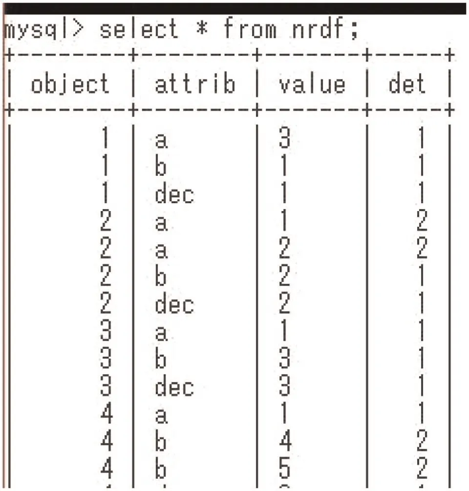
Fig. 9 Part of the NRDF format data set in Φ1

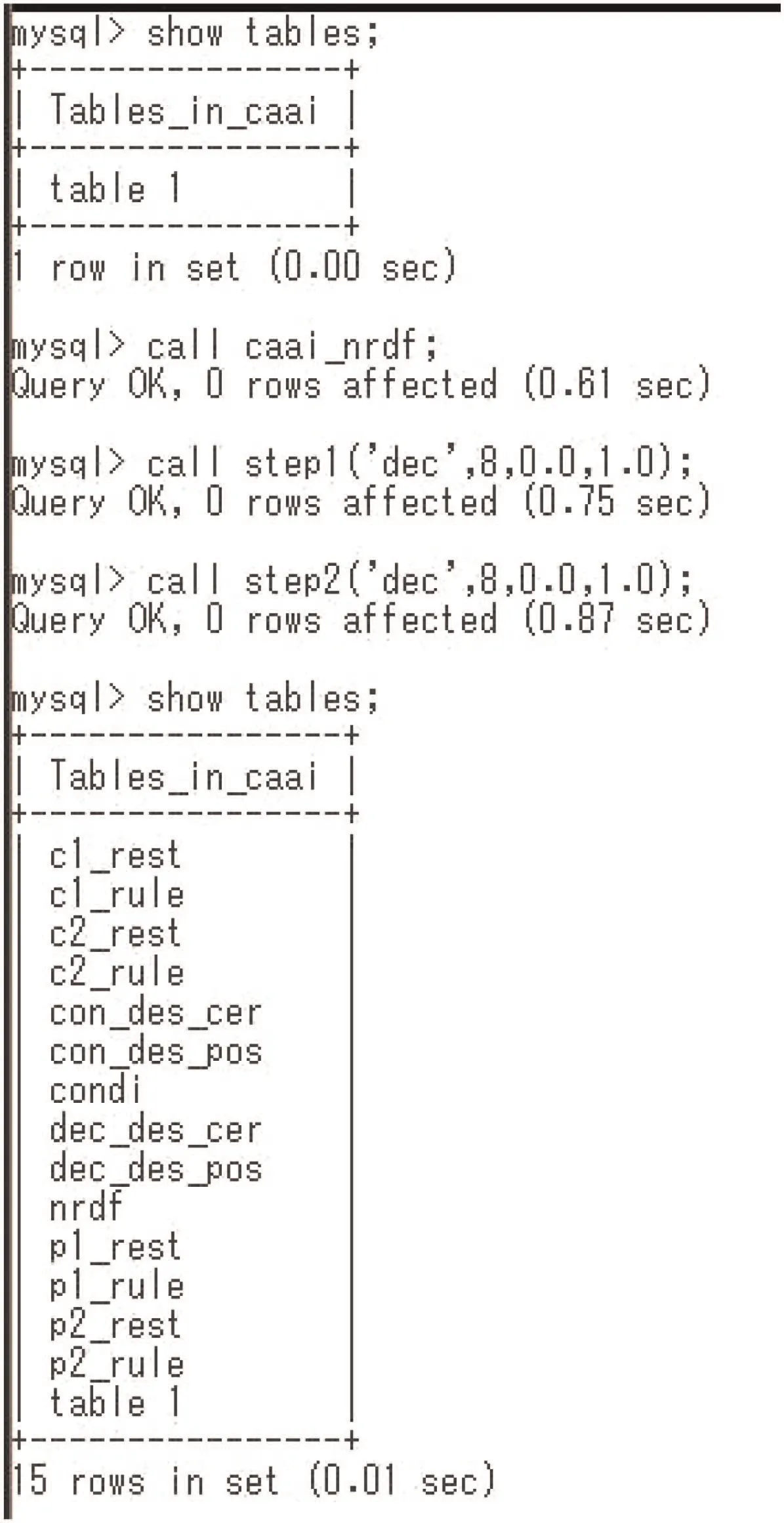
Fig. 10 Process of rule generation

6.2 Execution logs

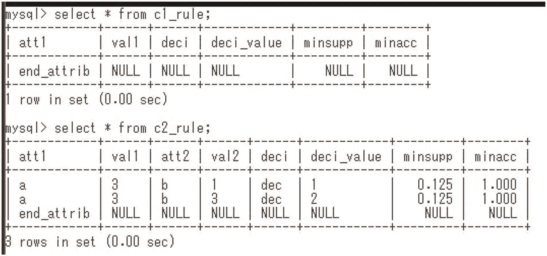
Fig. 11 Generated certain rules, which are shown in formula (1)

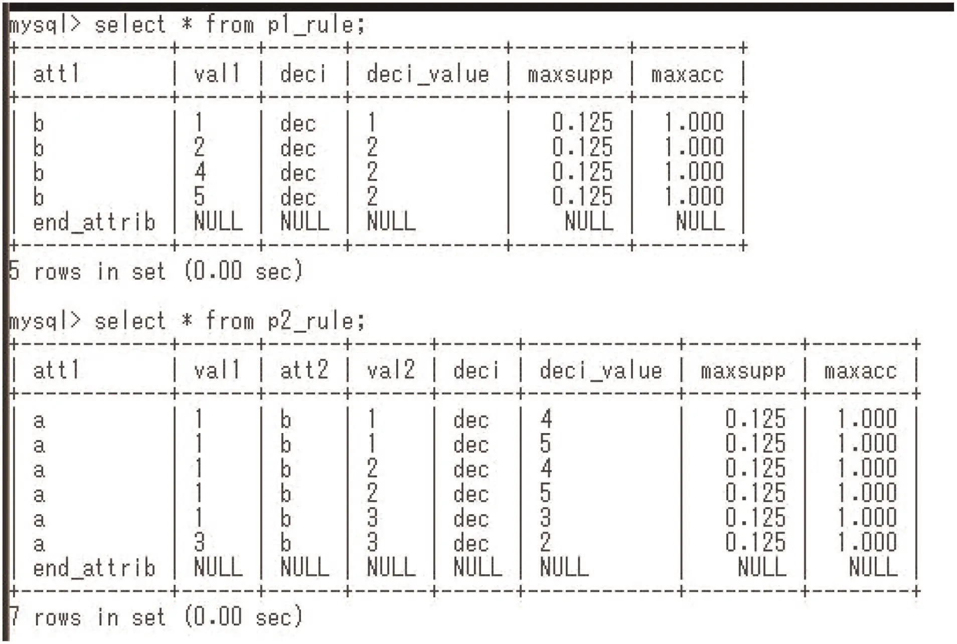
Fig. 12 Generated possible rules

We show NIS-Apriori-based rule generation in Fig. 10. At first,table 1 expressing Φ1is translated to the nrdf table by the caai_nrdf command. For the nrdf format tables, we can apply step1, step2, and step3 commands. They generate rules with one condition part, rules with two condition parts, and rules with three condition parts, respectively. In Fig. 10, step1 specifies the decision attribute is dec, support(τ)≥0.0 (any implication satisfies this constraint), and accuracy(τ)≥1.0. This specification means to generate minimal c-c rules in Definition 3. Fig. 11 shows the certain rules. These two certain rules are in formula (1) in Section 3.2. Fig. 12 shows the possible rules.

Other execution logs of the Mammographic data sets(|DD(Φ)|≥10100), the Credit Approval data sets (|DD(Φ)|≥1044), and the Congressional Voting data sets (|DD(Φ)|≥10100) [13], etc. are uploaded to [25].

7 Comparison of two types of rule generation and their combination

We reviewed two types of rule generation by using actual execution logs. Here, we summarise each role of rule generation (1A), (1B),(1C), (2A), (2B) in Section 1, again.

(1A) Rough set-based rule generation in DISs by the definability of a set X: A target set X specified by a descriptor [Dec,val]is given, and lower approximations of X are examined. Namely,accuracy(τ)=1.0 is employed as the top priority for rule generation. If we find an equivalence class [x]∧A∈CON[A,valA]?X,we have a consistent implication ∧A∈CON[A,valA]?[Dec,val].Thus, the problem to obtain consistent rule generation is translated to obtain a lower approximation of a set X.

(1B) Rough set-based rule generation in NISs by the definability of a set X:This is an extension of(1A),and the definability of a set X is extended to certainly definable and possibly definable due to information incompleteness. For handling two new definabilities,we employ search over the set of pe-classes with backtrack. If X is definable in each branch of search, X is certainly definable. If X is definable in at least one branch of search, X is possibly definable.We obtain some certain rules from certainly definable X and some possible rules from possibly definable X. Since the implemented program in Prolog employs exhaustive search, this program is not suitable for large size data sets.

(1C) Rough set-based rule generation in NISs by the discernibility function: The df-method is one of the algorithms to obtain a lower approximation of X specified by a descriptor [Dec,val]. This method translates the problem to obtain lower approximations into the SAT problem, and shows us a more comprehensive way to obtain lower approximations. Unfortunately, the SAT is NP-complete, therefore, the problem to obtain all lower approximations is NP-hard [11]. Even though we implemented a program in Prolog,which simulates a df-method for NISs,this program is not suitable for large size data sets.

(2A) DIS-Apriori-based rule generation: The Apriori algorithm generates every implication τ satisfying support(τ)≥α and accuracy(τ)≥β for 0 ＜α,β ≤1.0. We adjusted the Apriori algorithm for transaction data sets to table data sets, and termed it DIS-Apriori algorithm. The DIS-Apriori algorithm effectively uses support(τ) value, and sequentially generates candidates of rules.As a result, this algorithm has the same effect to examine each implication τ ∈∪i=1,...,(|AT|-1)IMPi. This causes completeness of the algorithm (any implication satisfying support(τ)≥α and accuracy(τ)≥β is detected by this algorithm). Since the Apriori algorithm is one of the representative algorithms of data mining,DIS-Apriori is useful for rule generation from table data sets. This algorithm is implemented in SQL.

(2B) NIS-Apriori-based rule generation: This algorithm is an extension of (2A), and the DIS-Apriori algorithm is extended to the NIS-Apriori algorithm for rule generation from NISs. We have proved some useful properties, and the NIS-Apriori algorithm can generate certain rules and possible rules from NISs. Even though the NIS-Apriori handles rules depending upon |DD(Φ)|, which may be more than 10100, the computational complexity is more than twice complexities of the DIS-Apriori algorithm and linear order complexity of the DIS-Apriori algorithm.

In rough set-based rule generation, rules concluding a descriptor[Dec,val] are obtained. So, we have to change a descriptor[Dec,val] sequentially for knowing all rules, and the support value of the obtained rule is additional. Implications with lower support value may be obtained. However, in Apriori-based rule generation, rules are characterised by the condition support(τ)≥α and accuracy(τ)≥β. Thus, we conclude the following:

(i) Apriori-based rule generation will be effective to know rules representing the tendency of the total data sets. Furthermore,soundness and completeness of the NIS-Apriori algorithm are proved. However, if we employ lower α, NIS-Apriori takes much execution time, because it cannot reduce the candidates of implication τ ∈∪i=1,...,(|AT|-1)IMPi. Namely, it is effective to obtain each rule with higher support value.

(ii) Rough set-based rule generation will be useful for obtaining rules, which show us the tendency of data sets. In rule generation,the support value of each implication is additional, and this value is calculated after finding lower approximations, so the support value does not affect the rule generation. The problem on the execution time in Apriori-based rule generation does not happen.However, the problem to obtain all rules is NP-hard, so completeness may not be assured.

To combine the advantage of two types rule generation, here we propose the NIS-Apriori algorithm with a target descriptor(tNIS-Apriori algorithm) in Algorithms 4 and 5 (see Figs. 13 and 14). We can easily generate tNIS-Apriori in SQL. We will employ NIS-Apriori in SQL for rule generation from the total data sets and tNIS-Apriori in SQL for rule generation from a part of a data set. The details of tNIS-Apriori in SQL, including the execution time, are in progress now.

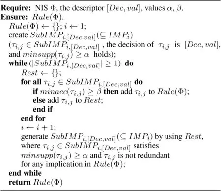
Fig. 13 Algorithm 4: NIS-Apriori algorithm with a target descriptor(certain rule generation part)

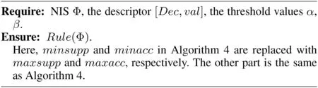
Fig. 14 Algorithm 5: NIS-Apriori algorithm with a target descriptor(possible rule generation part)

8 Conclusion

This paper reviewed our rule generators based on rough sets and the Apriori algorithm and clarified the property of each generator.NIS-Apriori in SQL can handle not only DISs but also NISs with information incompleteness, but the computational complexity will be the linear order complexity of the Apriori algorithm. As far as the authors know, NIS-Apriori in SQL is unique and a rare system with the preserving completeness of rule generation. This system does not miss any rules defined by the possible world semantics.We newly proposed a tNIS-Apriori algorithm for generating rules from a part of a data set. This comes from the combination of two types of rule generation.

To validate the proposing algorithms,cross-validation test is often employed [16]. There are many papers assuring the validity of algorithms by using this cross-validation test. However, soundness and completeness of defined rules assure the validity of the proposing algorithm. This is an advantage based on a logical framework. Of course,we also examined execution times, and they are in[25].

Rough sets seem to be defined for handling the concept of approximation, and rule generation is an application area of rough sets. Therefore, there are several types of research investigating lower and upper approximations without considering rule generation. We think it is necessary to aggregate such developed concepts of approximations to the actual rule generators. The tNIS-Apriori algorithm is an example of the integration of rough set-based rule generation and Apriori-based rule generation.

9 Acknowledgment

The first author expresses his special thanks to the organisers of the 2nd Asian Conference on AI Technology (June 8–10, 2018,Chongqing) for their inviting me to the keynote speech. This paper was partly supported by JSPS (Japan Society for the Promotion of Science) KAKENHI grant nos. 22500204 and 26330277.

10 References

[1] Pawlak, Z.: ‘Rough sets’, Int. J. Comput. Inf. Sci., 1982, 11, pp. 341–356

[2] Pawlak,Z.:‘Systemy informacyjne:podstawy teoretyczne’(WNT Press,Poland,1983), p. 186 (in Polish)

[3] Pawlak, Z.: ‘Rough sets’ (Kluwer Academic Publisher, Kluwer, Netherlands,1991)

[4] Lipski, W.: ‘On semantic issues connected with incomplete information databases’, ACM Trans. Database Syst., 1979, 4, (3), pp. 262–296

[5] Lipski, W.: ‘On databases with incomplete information’, J. ACM, 1981, 28, (1),pp. 41–70

[6] Or?owska, E., Pawlak, Z.: ‘Representation of nondeterministic information’,Theor. Comput. Sci., 1984, 29, (1–2), pp. 27–39

[7] Agrawal, R., Srikant, R.: ‘Fast algorithms for mining association rules in large databases’. Proc. VLDB’94, Morgan Kaufmann, 1994, pp. 487–499

[8] Ceglar, A., Roddick, J.F.: ‘Association mining’, ACM Comput. Surv., 2006, 38,(2), pp. 1–42, Article No. 5

[9] Sarawagi,S.,Thomas,S.,Agrawal,R.:‘Integrating association rule mining with relational database systems: alternatives and implications’, Data Min. Knowl.Discov., 2000, 4, (2), pp. 89–125

[10] Komorowski,J.,Pawlak,Z.,Polkowski,L.,et al.:‘Rough sets:a tutorial’,in Pal,S.K.,Skowron,A.(Eds.):‘Rough fuzzy hybridization:a new method for decision making’ (Springer, German, 1999), pp. 3–98

[11] Skowron, A., Rauszer, C.: ‘The discernibility matrices and functions in information systems’, in S?owiński, R. (Ed.): ‘Intelligent decision support –handbook of advances and applications of the rough set theory’ (Kluwer Academic Publishers, Netherlands, 1992), pp. 331–362

[12] Kripke, S.A.: ‘Semantical considerations on modal logic’, Acta Philos. Fenn.,1963, 16, pp. 83–94

[13] ‘UCI machine learning repository’. Available at http://mlearn.ics.uci.edu/MLRepository.html, accessed April 2010

[14] Sakai, H., Wu, M., Nakata, M.: ‘Apriori-based rule generation in incomplete information databases and non-deterministic information systems’, Fundam.Inf., 2014, 130, (3), pp. 343–376

[15] Sakai, H., Nakata, M., Watada, J.: ‘NIS-Apriori-based rule generation with three-way decisions and its application system in SQL’,Inf.Sci.,2018(in Press)

[16] Tsumoto,S.:‘Automated extraction of medical expert system rules from clinical databases based on rough set theory’, Inf. Sci., 1998, 112, pp. 67–84

[17] Ziarko,W.:‘Variable precision rough set model’,J.Comput.Syst.Sci.,1993,46,(1), pp. 39–59

[18] Ciucci, D., Flaminio, T.: ‘Generalized rough approximations in PI 1/2’,Int. J. Approx. Reason., 2008, 48, (2), pp. 544–558

[19] Greco,S.,Matarazzo,B.,S?owiński,R.:‘Granular computing and data mining for ordered data: the dominance-based rough set approach’, in Meyers, R.A. (Ed.):‘Encyclopedia of complexity and systems science’ (Springer, USA, 2009),pp. 4283–4305

[20] Grzyma?a-Busse, J.W.: ‘Data with missing attribute values: generalization of indiscernibility relation and rule induction’, Trans. Rough Sets, 2004, 1,pp. 78–95

[21] Kryszkiewicz,M.:‘Rough set approach to incomplete information systems’,Inf.Sci., 1998, 112, (1–4), pp. 39–49

[22] Miao, D., Zhao, Y., Yao, Y., et al.: ‘Relative reducts in consistent and inconsistent decision tables of the Pawlak rough set model’, Inf. Sci., 2009,179, (24), pp. 4140–4150

[23] Nakata, M., Sakai, H.: ‘Twofold rough approximations under incomplete information’, Int. J. Gen. Syst., 2013, 42, (6), pp. 546–571

[24] Qian,Y.H.,Liang,J.Y.,Yao,Y.Y.,et al.:‘MGRS:a multi-granulation rough set’,Inf. Sci., 2010, 180, pp. 949–970

[25] Sakai,H.:‘Execution logs by RNIA software tools’.Available at http://www.mns.kyutech.ac.jp/sakai/RNIA, accessed January 2016

[26] Wang, G.: ‘DGCC: data-driven granular cognitive computing’, Granular Comput., 2017, 2, pp. 343–355

[27] Wu,W.Z.,Mi,J.S.,Zhang,W.X.:‘Generalized fuzzy rough sets’,Inf.Sci.,2003,151, pp. 263–282

[28] Yao, Y.Y.: ‘Three-way decisions with probabilistic rough sets’, Inf. Sci., 2010,180, pp. 314–353

[29] Yao, Y.Y., She, Y.: ‘Rough set models in multigranulation spaces’, Inf. Sci.,2016, 327, pp. 40–56

[30] Zhang,Q.,Xie,Q.,Wang,G.:‘A survey on rough set theory and its applications’,CAAI Trans. Intell. Technol., 2016, 1, (4), pp. 323–333

[31] Codd, E.F.: ‘A relational model of data for large shared data banks’, Commun.ACM, 1970, 13, (6), pp. 377–387

[32] Grzyma?a-Busse,J.W.,Werbrouck,P.:‘On the best search method in the LEM1 and LEM2 algorithms’, Stud. Fuzziness Soft Comput., 1998, 13, pp. 75–91

[33] Sakai, H.: ‘Effective procedures for handling possible equivalence relations in non-deterministic information systems’,Fundam.Inf.,2001,48,(4),pp.343–362

[34] Sakai, H., Okuma, A.: ‘Basic algorithms and tools for rough non-deterministic information analysis’, Trans. Rough Sets, 2004, 1, pp. 209–231

[35] Sakai, H., Okuma, H., Wu, M., et al.: ‘Rough non-deterministic information analysis for uncertain information’, in Nakamatsu, K., Jain, L.C. (Eds.): ‘The handbook on reasoning-based intelligent systems’ (World Scientific, Singapore,2013), pp. 81–118

[36] Sakai, H., Nakata, M.: ‘An application of discernibility functions to generating minimal rules in non-deterministic information systems’, J. Adv. Comput.Intell. Intell. Inf., 2006, 10, (5), pp. 695–702

[37] Sakai, H., Ishibashi, R., Koba, K., et al.: ‘Rules and apriori algorithm in non-deterministic information systems’, Trans. Rough Sets, 2008, 9,pp. 328–350

[38] Sakai, H., Liu, C., Zhu, M., et al.: ‘On NIS-Apriori based data mining in SQL’. Proc. Int. Conf. Rough Sets, 2016 (LNCS, 9920),pp. 514–524

[39] ?le?zak, D., Sakai, H.: ‘Automatic extraction of decision rules from non-deterministic data systems: theoretical foundations and SQL-based implementation’. Proc. DTA 2009, 2009, vol. 64, pp. 151–162

[40] ?le?zak, D., Eastwood, V.: ‘Data warehouse technology by infobright’.Proc. ACM SIGMOD, 2009, pp. 841–846

[41] Kowalski, M., Stawicki, S.: ‘SQL-based heuristics for selected KDD tasks over large data sets’. Proc. FedCSIS 2012, 2012, pp. 303–310

[42] Swieboda,W.,Nguyen,S.:‘Rough set methods for large and spare data in EAV format’. Proc. IEEE RIVF, 2012, pp. 1–6