Changming Zhu, Duoqian Miao ?

1College of Information Engineering, Shanghai Maritime University, No. 1550, Haigang Avenue, Shanghai, People’s Republic of China

2Department of Computer Science and Technology, Tongji University, No. 4800, Cao’an Highway, Shanghai, People’s Republic of China

Abstract:Classical radial basis function network(RBFN)is widely used to process the non-linear separable data sets with the introduction of activation functions. However, the setting of parameters for activation functions is random and the distribution of patterns is not taken into account. To process this issue, some scholars introduce the kernel clustering into the RBFN so that the clustering results are related to the parameters about activation functions. On the base of the original kernel clustering, this study further discusses the influence of kernel clustering on an RBFN when the setting of kernel clustering is changing. The changing involves different kernel-clustering ways [bubble sort (BS) and escape nearest outlier (ENO)], multiple kernel-clustering criteria (static and dynamic) etc. Experimental results validate that with the consideration of distribution of patterns and the changes of setting of kernel clustering, the performance of an RBFN is improved and is more feasible for corresponding data sets. Moreover, though BS always costs more time than ENO, it still brings more feasible clustering results. Furthermore, dynamic criterion always cost much more time than static one, but kernel number derived from dynamic criterion is fewer than the one from static.

1 Introduction

Neural network (NN), which is also called artificial NN (ANN) [1,2], is a mathematical or computational model. There are many kinds of ANNs. In terms of learning algorithms, supervised or unsupervised learning networks [3, 4], hybrid learning networks [5],associate learning networks [6], and optimisation application networks [7] are used widely. In terms of network connectionism,feed-forward networks [8], recurrent networks [9], and reinforcement networks [10] are used widely. Regardless of which kind of network is used, the structure of a network always consists of three parts: input layer, hidden layer, and output layer. In the hidden layer, mapping functions are called activation functions.Kernel functions are always treated as activation functions. The most well known activation functions are radial basis functions(RBFs) which are also treated as RBF kernels. A network with RBF kernels is named an RBF network (RBFN). RBFN is a linear combination of RBF kernels. RBF kernels have two parameters,centres, and radiuses (or widths). They are determined by unsupervised or supervised learning [11, 12]. In RBFN, the connection weights between hidden units and output units and the thresholds of output units are adjusted by supervised learning rules. Similar to multi-layered perception (MLP), supervised learning rules of RBFN such as steepest descent method can be applied to minimise the sum of squared errors, which are the differences between the inference outputs of the model and the desired outputs. In unsupervised learning, the mean of patterns, determined with K-means algorithms, can be used as the centre of kernel, and then one can determine the appropriate size of the radius with the nearest neighbour rule [12].

The activation function of RBFN is given by the following equation:

where L is the number of hidden units and x is an input feature vector, namely, pattern. μjand σjare centre and radius of the jth RBF kernel Kj, respectively.

In the original RBFN, activation functions always have a same setting and without the consideration of data structure. This makes patterns in an L-dimensional space have no feasible distribution though they are linear separable. From work [13], Gao and Li proposed a new kernel nearest neighbour classification method, such that a pattern is labelled according to the minimum distance between itself and the surfaces of the existing kernels. We can adopt their kernel-generating method to gain more feasible kernels for RBFN.In fact,there are many factors that should be considered during the process of the generation of kernels.This paper proposes a new kind of kernel-clustering method.Our basic ideas differ from the one given in[13].Here,different kernel criteria and ways,ways of the computation of kernel centre,and width should be taken into account. Finally, experimental results on Letter, Pen digit, Shuttle,US Postal Service (USPS), Iris, and Two Spiral demonstrate the effectiveness of the proposed method.

2 Related work

2.1 Original kernel clustering

Gao and Li [13]propose a kernel nearest neighbour method,which aims to label a pattern according to the minimum distance between itself and the surfaces of the existing kernels. In [13], a kernel is treated as a cluster and the process is given below:

(i)For a data set,we first choose a class as the object class and select a pattern as the initial centre for a kernel. Here, the class being clustered is called the object class. Corresponding patterns of this class are called object patterns. Other classes are called non-object classes and the corresponding patterns are called outliers or non-object patterns.

(ii) We compute the minimum Euclid distance between patterns from the object class and non-object class and the centre of the present object kernel and denote the two distances as d1aand d1b.The corresponding patterns are denoted as x1aand x1b.

(iii)If d1a＜d1b,put x1ainto this kernel and then update the kernel.Otherwise, stop growing the kernel and choose the next position to generate a new object kernel. In [13], for the updated kernel, we should first update the centre. The new centre is the mean of new object patterns in this kernel. Then, compute the new d1aand d1b.The updated width is the mean of new d1aand d1b; specifically,Widthker=(d1a+d1b/2).

(iv)Repeat steps(ii)and(iii),we cover class CAby KAkernels,until all patterns from the training subsets in this object class are covered by different kernels.

In our method, we use this kernel-clustering method as the basic algorithm and provide some new ideas to improve it.

2.2 Computation about kernel centre and radius of a Gaussian unit

RBF is always defined as a monotonic function of the Euler distance from point x in the input space into a centre xcand it can be denoted as k(‖x-xc‖);the function is local:namely,when x is far from xc,the value is small. The most widely used RBF is written as k(‖x-xc‖)=e-(‖x-xc‖/2σ2), where xcis the centre of a kernel, σ is its width and it controls the area of radius function. In RBFN,these two parameters can be changed. Some methods are widely used:

(i)To select the centre based on experience.For example,as long as the distribution of training patterns can represent a given problem,we can select M centres based on experience of the uniform distribution, and the spacing is d, the width of the Gaussian kernel function is σ

(ii) To select the basis function by a clustering method. We can put the cluster centres as the centres of basis functions, with the variance of the various types of patterns as the width parameters of each basis function. After determining the parameters of the hidden layer of basis functions, as the output layer is a linear unit,its weight can simply be calculated directly using the least-squares method.

(iii) The centre, width, and weights can be calculated by an errorcorrection algorithm through the training patterns. The practise is similar with BP, which is used to calculate the derivatives of the error e(k) parameters of parameters, and then use iteration to determine the parameters. We can fix centres and widths, only to learn the weight values.

3 New kernel clustering

Here, we change the setting of the original kernel clustering and develop a new kernel clustering. The changes involve different ways for kernel clustering and their criteria, and different computation ways about kernel centres and widths. Then, we apply newly generated kernels into RBFN.

The basic steps of this new method are similar with the original one, namely, choose the initial centre, compute the distance,cover the object patterns, and update the kernels. The differences are that in our method, we use different kernel-clustering ways and criteria to generate kernels. The widths of kernels have other equations for computation. The algorithm will stop until all object patterns in each class have been covered by different kernels. The framework of our work is given in Fig. 1. From this table, it is found that the algorithm has at least three parameters and in terms of RBFN, different parameters will bring different performances.

3.1 Computation of kernel centre and width

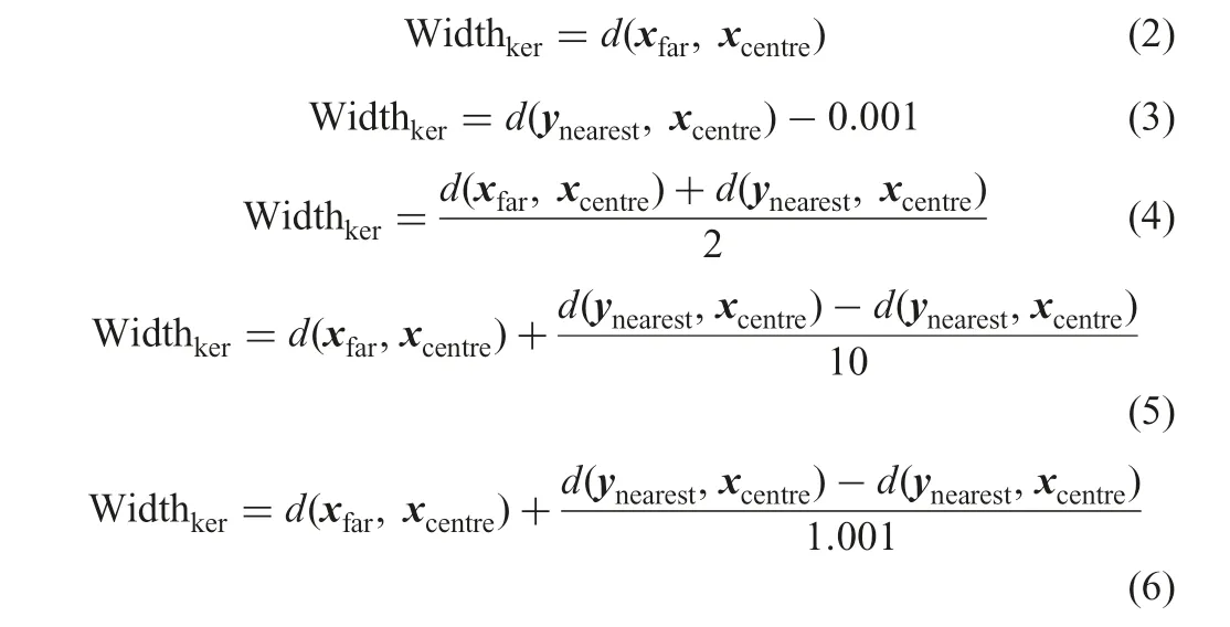
Here, d(xfar, xcentre) denotes the furthest distance between patterns in the object class and the centre of the present kernel while d(ynearest, xcentre) means the nearest distance between patterns from non-object classes and the centre of the present kernel. Then, we adopt the following five ways to determine the width of kernel.Equation (4) gives the method, which is used in the original way.

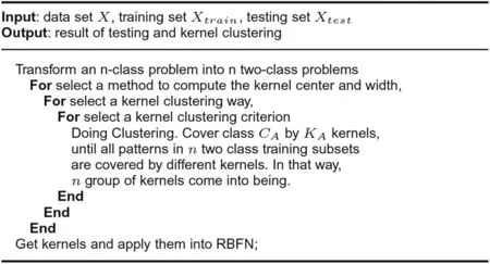
Fig. 1 Algorithm: kernel clustering

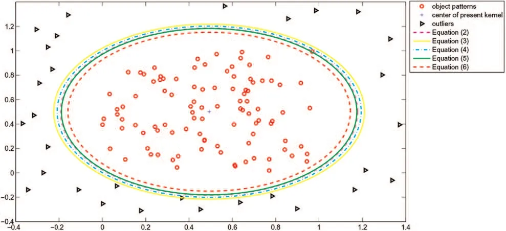
Fig. 2 Differences between five ways to compute the width of the kernel

Fig. 2 shows the differences between these five ways. From the outer to the inner are five width contours with (2)–(6). From the contours, we find that (2) and (5) make kernel tight, (3) makes it somewhat loose, and (4) is moderate while (6) is so small as not to cover all object patterns. Furthermore, (6) can decrease the chance of misclassifying testing patterns because the width radius is diminished

3.2 Kernel-clustering method

Two kinds of kernel-clustering ways are adopted here.One is bubble sort (BS) and the other is escape nearest outlier (ENO).

BS aims to cover object patterns one by one. In BS, it computes the minimum distance between patterns from object class and non-object class and the centre of the present object kernel Then it compares the two distances so as to decide whether to include this new object pattern into present kernel or not. If yes, cover the new pattern and update the kernel; otherwise, stop growing the present kernel and choose a next position to generate a new object kernel.

ENO aims to generate one object kernel by computing the nearest distance between patterns from non-object classes and the centre of the present kernel.This distance is denoted as d1b.Then,ENO puts all object patterns whose distance to the centre is less than d1binto the object kernel. The centre of this kernel is not changed and the width can be updated with (2)–(6).

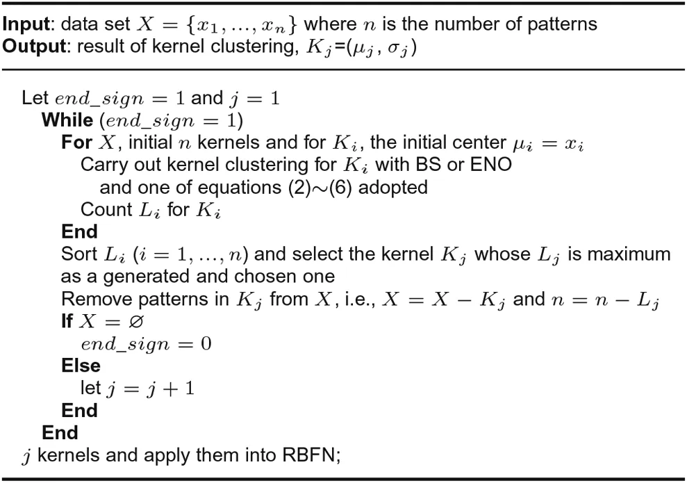
Fig. 3 Algorithm: dynamic kernel clustering

BS generates kernels well, but it costs too much time to cover object patterns one by one. ENO contrasts with BS in terms of these performances. However, we should note that the number of kernels with BS or ENO has no absolute relationship.

3.3 Kernel-clustering criteria

Two kinds of kernel-clustering criteria are adopted in our work.One is static criterion and the other is dynamic criterion.

The static kernel clustering is similar with the original kernel clustering (please see Section 2.1) and the only difference is the different way to compute kernel widths. Static kernel clustering adopts (2)–(6) to compute the kernel widths while the original kernel clustering adopts ways given in Section 2.2 to compute kernel widths.

Table 1 Experimental setting

Compared to the static kernel clustering,dynamic one is more complicated and its steps are given in Fig.3.In this table,xiindicates the ith pattern and Kjis the jth kernel.Liis‘left index’and it indicates the total number of patterns which are only covered by Ki.

From steps of these two criteria,it is found that dynamic criterion is more time-consuming.However,with dynamic criterion,the number of kernels is fewer since in dynamic kernel clustering, we choose a kernel, which can cover maximum patterns uniquely at each time.

4 Experiment

To validate the effectiveness of our work,we adopt data sets Letter,Pen digit, Shuttle, USPS, Iris, and Two Spiral for experiments, and then we provide further discussion in terms of (i) differences between BS and ENO, (ii) differences between static and dynamic criteria, (iii) convergence analysis, (iv) generalisation risk analysis,and (v) the testing results of RBFN with different kernel-clustering ways and the comparison between our method and others.

4.1 Experimental setting

The experiment setting is shown in Table 1.Main numerical characteristics are summarised in Table 2.Here,columns A–M denote data set,number of training set, number of testing set, number of classes,number of attributes, the maximum data of training set, the minimum data of training set,the mean of training set,the co-variance of training set,the maximum data of testing set,the minimum data of testing set,the mean of testing set,and the co-variance of testing set.Our experimental environment is simple and crude.All computations are performed on Pentium D processor with 2.66 GHz,512 M RAM,Microsoft Windows XP,and MATLAB 7.0 environment.This configuration leads to somewhat long computations.However,this does not influence conclusions derived from the experiments.

4.2 Kernel-clustering results

Here,we use Letter,Pen digit,Shuttle,USPS,Iris,and Two Spiral to show the effectiveness of the proposed kernel-clustering method.We adopt different kernel-clustering ways, criteria, and ways to compute kernel centres and widths so as to get kernel-clustering results.Table 3 gives the combinations of these different parameters.Table 4 gives the corresponding kernel results. From the results, we find that the results are better than those in [13] in average. It is found that BS always costs much more time than ENO,but BS generates more feasible kernels.What is more,dynamic criterion always cost much more time than static one,but with dynamic criterion,the kernel number is smaller than the one with static criterion.

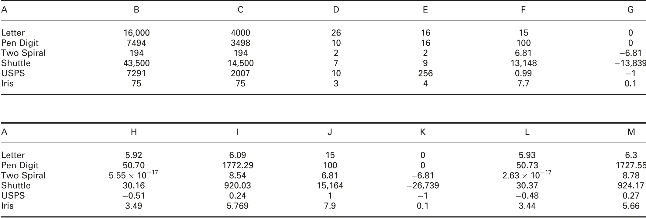
Table 2 Basic characteristics of Letter,Pen Digit, Shuttle, USPS, Iris, PID, Two Spiral, and 2D-VOW data sets

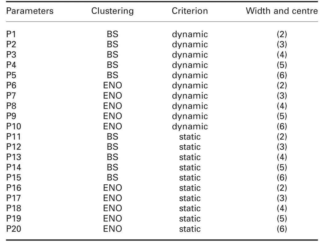
Table 3 Parameter configurations

4.3 Further discussion

We also give some further discussion in terms of the following five parts:

(i) The difference between BS and ENO: In fact, in the previous experiments, we can find that BS can generate more feasible kernels than ENO does, while it costs much more time compared with ENO.

(ii) The difference between static and dynamic criterion: Static criterion saves time for kernel clustering while dynamic criterion can generate fewer kernels.

(iii)For assessing the effectiveness of a classifier,two criteria should be adopted.One is convergence and the other is generalisation risk.We adopt these two criteria so as to validate the effectiveness of the proposed method.

(iv) Testing results of RBFN with different kernel-clustering ways:From the results, we find that for most cases, results under the new RBF are better than those without RBF. Comparisons between our method and other methods, for example, Na?ve Bayes[14, 15], AdaBoost [16] (the standard ensemble algorithm), C4.5[17, 18] (the most popular decision tree method), K-means method[19] (for determining the hidden structure directly), the k-nearest neighbour algorithm (KNN) [19], MLP [20] (a method that uses back propagation to estimate RBFNN), and probabilistic NN(PNN) [21] are also given.

4.3.1 Difference between BS and ENO: In our proposed method, we use two kernel-clustering ways: BS and ENO. In terms of some data sets, Table 5 gives time of kernel clustering with these two methods. First, for USPS, Letter, and Two Spiral,we use static criterion, and in terms of the computation of width,we adopt (2). For Pen digit, we use static criterion, and adopt (5)as the way to compute the width. For Iris, static criterion and (6)are adopted. In terms of Shuttle, we use ENO, dynamic criterion,and (2) is used to compute the widths and centres of kernels.

Time of kernel clustering for BS and ENO and corresponding numbers of kernels are shown in Table 5. From this table, we find that ENO can save more time than BS. However, BS generates fewer kernels than ENO does. The reason is that in terms of BS, the centre of a kernel is changed when a new object pattern comes. It should update the centre and width of this kernel each time when the new object pattern has been covered. However, in the process of ENO, the centre will not be changed and we regard the initial pattern as the kernel centre.

4.3.2 Difference between static and dynamic criteria: Table 6 gives the best numbers of kernels with different kernel parameters and data sets. From this table, we find that though dynamic criterion costs more clustering time than static one, with dynamic one, the number of kernels is not more than or fewer than one with static criterion. From the principles of the two criteria, we know that dynamic criterion aims to choose kernels whose ‘left indexes’ are large enough to cover all object patterns. This is a ‘positive’ way. However, static criterion only uses the way, which is similar with the original kernel clustering to generate kernels. In contrast, dynamic one is more time-consuming than static one, because under dynamic one, we should make each pattern of object class be an initial centre of a kernel and compute the ‘left index’.

4.3.3 Convergence analysis: For assessing the effectiveness of a classifier,two criteria should be adopted.One is convergence and the other is generalisation risk. Here, we adopt an empirical justification given in [22], so as to demonstrate that all compared methods can converge within limited iterations. Table 7 shows the numbers of iterations for these methods on all used data sets.

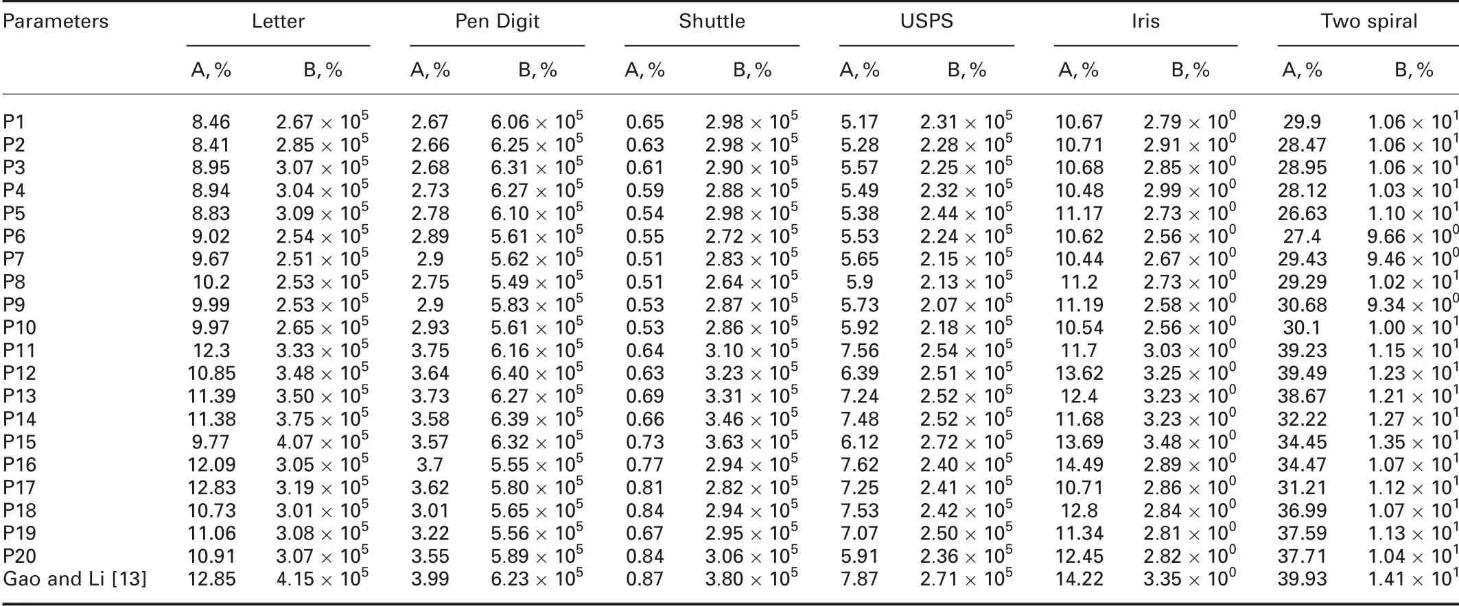
Table 4 Kernel-clustering results

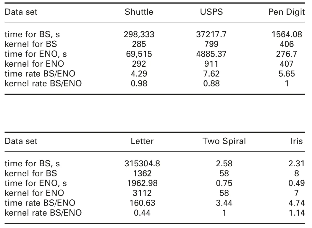
Table 5 Time of kernel clustering for BS and ENO

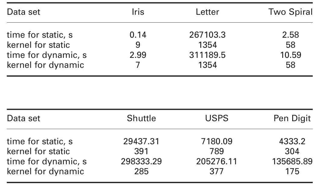
Table 6 Time of kernel clustering for static and dynamic criteria

From this table,it is found that the proposed method can converge in fewer iterations. This also means that the method has a simple structure.

4.3.4 Generalisation risk analysis: As one of the criteria to assess effectiveness of a method, the analysis of generalisation risk is important for interpreting the performance behaviour of a method. If the generalisation risk of a method is smaller, this method has a lower prediction error on label-unknown patterns. In[23], some researchers have interpreted it and given an algorithm about how to compute the generalisation risk of a method in statistics rather than compute the value of the objective function simply. Here, we still use the same way to compute the generalisation risk of the proposed method. Table 8 shows generalisation risks for all compared methods. From this table, in terms of the average generalisation risk, it is found that the proposed method has a smaller generalisation risk than others in average. This also means that the proposed method has a better prediction ability to label the testing patterns.

4.3.5 Testing results of RBFN with different kernel-clustering ways and the comparison between our method and others: Finally, we give the results of RBFN with our proposed method and the original way in Table 9. The average classification performances of our method and other methods are also given in this table.

Then,with a data set used,the process of selecting the best parameters of a compared method includes the following four steps:(i) except for the constant parameters, the methods used here have some adjustable parameters and different values of them affect the experimental results. Then, for each method, according to its corresponding parameters,we choose different initial values of them so as to generate all combinations of the corresponding parameters;(ii)for a combination of each method’s corresponding parameters, we use one group of training patterns to train a temporary model and then use this trained model to classify the corresponding testing patterns so as to get the corresponding classification accuracy;(iii)under the case of this combination of the parameters,the process in the previous step is repeated ten times according to the corresponding ten groups of training and testing sets and ten corresponding classification performances are gotten.Then,we obtain the average classification accuracy, which is regarded as the experimental result of the present combination of the parameters; and (iv) for a method, after implementing all possible combinations of its corresponding parameters,we get their corresponding average classification performances. Among the performances, we choose the best one and the corresponding parameters are regarded as the best ones. Then, the corresponding average classification accuracy with the best parameters is regarded as the final experimental result for the classification problem of the data set with the method used.

Table 7Numbers of iterations comparisons for all compared methods on all data sets

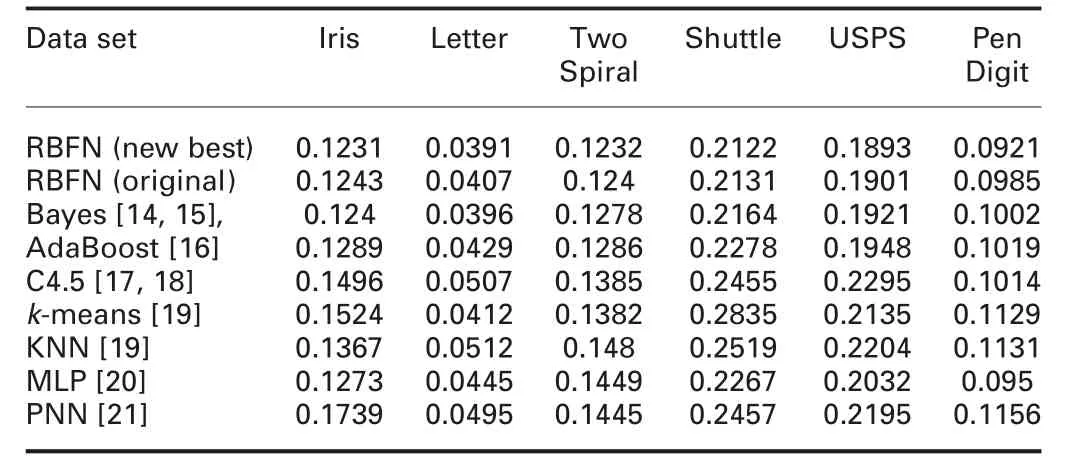
Table 8 Generalisation risk comparison

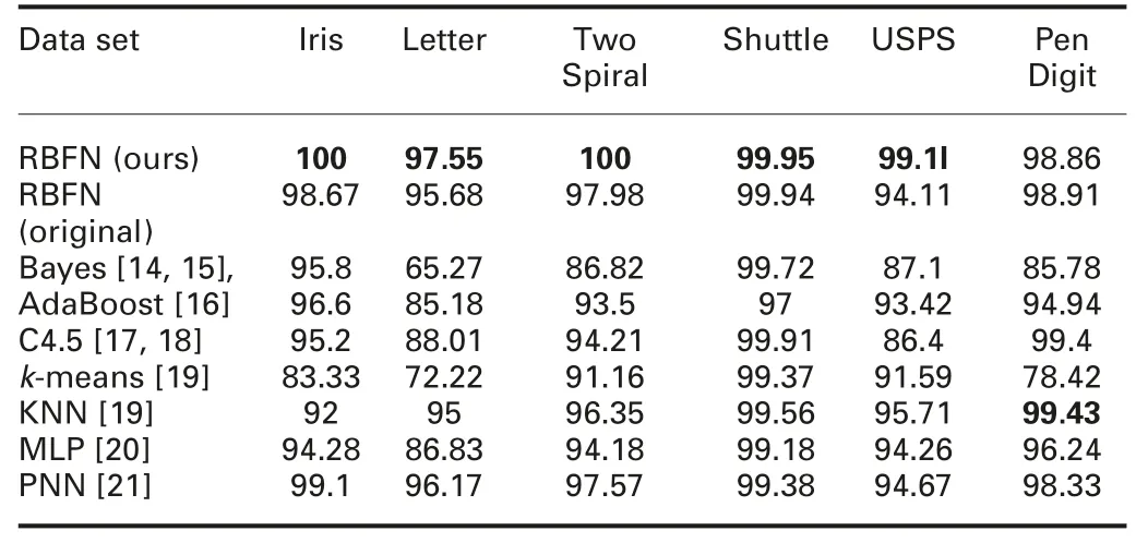
Table 9 Average classification performances of our method and other methods

Then,for the classification problem of a data set,as we used many compared methods, we repeat the process for each one until we set the best parameters for all methods used here. As a result, we can also get the final classification performances of them for the classification problem.

From these results, we find that after the process of our method,RBFN with the new generated kernels has a better performance under most cases. In fact, new kernels bring better activation functions to map the patterns into a kernel space.

5 Conclusion

In this paper, we propose a new RBFN, which is based on a new kernel-clustering method. We consider many fields of kernel clustering and set different kinds of parameters about kernel clustering. Experiments have validated the influence of the parameters on the classification accuracy and time for clustering.In our work, we give some further discussion about (i) differences between BS and ENO, (ii) differences between static and dynamic criteria, (iii) convergence analysis, (iv) generalisation risk analysis,and (v) testing results of RBFN with different kernel-clustering ways and the comparison between our method and others.

From these results, it is found that with kernel clustering, the classification performance becomes better than the original algorithm. Different parameters and ways bring different classification results. The most important matters derived from our experiments are (i) BS always costs more time than ENO, but BS has feasible kernels, (ii) dynamic criterion always costs more time than static one, but dynamic one brings fewer kernels.

For our proposed method,we should learn that to achieve a better performance for classification, kernel clustering is necessary. In kernel clustering, different clustering parameters lead to different kernel results. Then, BS and dynamic criterion are the first choice for kernel clustering when the data set is not very large. If we process a large-scale data set, static criterion and ENO is a good choice. We should know, in terms of classification that BS and ENO will not bring a great difference. However, if we want to have more feasible kernels, BS is better than ENO. If we want to have fewer kernels, dynamic criterion is superior to static one.ENO and static criterion save time versus BS and dynamic one.

In the future,we will find a good method that can save more time for clustering and bring fewer and more feasible kernels. We will also use more large-scale data sets in future experiments.

6 Acknowledgments

This work was sponsored by the‘Chenguang Program’supported by the Shanghai Education Development Foundation and Shanghai Municipal Education Commission under Grant no. 18CG54.Furthermore, this work was also supported by the National Natural Science Foundation of China (CN) under Grant nos. 61602296 and 61673301; the Natural Science Foundation of Shanghai (CN)under Grant no. 16ZR1414500; Project funded by the China Postdoctoral Science Foundation under Grant no. 2019M651576;the National Key R&D Program of China (Grant no. 213), and the authors thank their supports.

7 References

[1] Yang, Z.B., Lin, D.K.J., Zhang, A.J.: ‘Interval-valued data prediction via regularized artificial neural network’, Neurocomputing, 2019, 331,pp. 336–345

[2] Lu, L., Yu, Y., Yang, X.M., et al.: ‘Time delay Chebyshev functional link artificial neural network’, Neurocomputing, 2019, 329, pp. 153–164

[3] Liu, J., Gong, M.G., He, H.B.: ‘Deep associative neural network for associative memory based on unsupervised representation learning’, Neural Netw., 2019,113, pp. 41–53

[4] Oh,C.,Ham,B.,Kim,H.,et al.:‘OCEAN:object-centric arranging network for self-supervised visual representations learning’, Expert Syst. Appl., 2019, 125,pp. 281–292

[5] Adhikari, S.P., Yang, C.J., Slot, K., et al.: ‘Hybrid no-propagation learning for multilayer neural networks’, Neurocomputing, 2018, 321, pp. 28–35

[6] Stahlbuhk, T., Shrader, B., Modiano, E.: ‘Learning algorithms for scheduling in wireless networks with unknown channel statistics’, Ad Hoc Netw., 2019, 85,pp. 131–144

[7] Jin, L., Li, S., Hu, B.: ‘A survey on projection neural networks and their applications’, Appl. Soft Comput., 2019, 76, pp. 533–544

[8] Yang, J., Ma, J.: ‘Feed-forward neural network training using sparse representation’, Expert Syst. Appl., 2019, 116, pp. 255–264

[9] Zia,T.:‘Hierarchical recurrent highway networks’,Pattern Recognit.Lett.,2019,119, pp. 71–76

[10] Yao,H.P.,Chen,X.,Li,M.Z.,et al.:‘A novel reinforcement learning algorithm for virtual network embedding’, Neurocomputing, 2018, 284, pp. 1–9

[11] Líczaro, M., Hayes, M. H., Figueiras-Vidal, A.R.: ‘Training neural network classifiers through Bayes risk minimization applying unidimensional Parzen windows’, Pattern Recognit., 2018, 77, pp. 204–215

[12] Gadaleta, M., Rossi, M.: ‘IDNet: smartphone-based gait recognition with convolutional neural networks’, Pattern Recognit., 2018, 74, pp. 25–37

[13] Gao, D.Q., Li, J.: ‘Kernel fisher discriminants and kernel nearest neighbor methods: a comparative study for large-scale learning problems’. Int. Joint Conf. Neural Networks, 2006, pp. 1333–1338

[14] Jiang,L.X.,Zhang,L.G.,Yu,L.J.,et al.:‘Class-specific attribute weighted Na?ve Bayes’, Pattern Recognit., 2019, 88, pp. 321–330

[15] Harzevili, N.S., Alizadeh, S.H.: ‘Mixture of latent multinomial naive Bayes classifier’, Appl. Soft Comput., 2018, 69, pp. 516–527

[16] Lee,W.,Jun,C.H.,Lee,J.S.:‘Instance categorization by support vector machines to adjust weights in AdaBoost for imbalanced data classification’,Inf.Sci.,2017,381, pp. 92–103

[17] Han,L.,Li,W.J.,Su,Z.:‘An assertive reasoning method for emergency response management based on knowledge elements C4.5 decision tree’, Expert Syst.Appl., 2019, 122, pp. 65–74

[18] Kudla, P., Pawlak, T.P.: ‘One-class synthesis of constraints for mixed-integer linear programming with C4.5 decision trees’, Appl. Soft Comput., 2018, 68,pp. 1–12

[19] Ismkhan, H.: ‘I–k-means?+: an iterative clustering algorithm based on an enhanced version of the k-means’, Pattern Recognit., 2018, 79, pp. 402–413

[20] Mondal, A., Ghosh, A., Ghosh, S.: ‘Scaled and oriented object tracking using ensemble of multilayer perceptrons’, Appl. Soft Comput., 2018, 73,pp. 1081–1094

[21] Kusy, M., Kowalski, P.A.: ‘Weighted probabilistic neural network’, Inf. Sci.,2018, 430-431, pp. 65–76

[22] Ye, J.: ‘Generalized low rank approximations of matrices’, Mach.Learn., 2005,61, (1–3), pp. 167–191

[23] Scholkopf, B., Taylor, J.S., Smola, A., et al.: ‘Generalization bounds via eigenvalues of the gram matrix’. Technical Report 1999–035, 1999,NeuroColt