Farhad Sakhaee

School of Engineering, Parks College of Engineering, Aviation and Technology, Saint Louis University, USA

Abstract An unstructured mesh has been developed to simulate both steady and unsteady flow conditions over a spillway.Discretization has been done based on finite volume method for a two-dimensional depth averaged model.Different hydraulic parameters such as water depth profile, velocity, Froude number, shear stress were calculated and presented in detail for both scenarios.Finally, Normalized Shields distribution calculated wherein areas prone to deposition and erosion were estimated accordingly.SRH-2D Model were used as a hydrodynamic tool to investigate the effects of steady and unsteady state flow conditions overflown over the spillway of a dam.Flood plain delineation is crucial both at coastal areas as well as river neighborhood structures.In either case, it will give us a strong sense of buffer zone estimation.This buffer zone acts as a safety distance from the flood in case of water crises.

Keywords: Numerical Simulation; 2D-Model; Normalized Shields Distribution; Deposition; Erosion.

1.Introduction

1-D models are applicable when a long reach (more than 50 km) is investigated over a long period.On the other hand, 3D modeling with Naiver-Stokes equations is necessary when a hydraulic structure is located at the adjacent areas.Hence a 2-D depth averaged model is considered for most of prac- tical open channel moldings [1] .Young et al., 2011, studied the bedrock erosion based on a two-dimensional depth aver- aged model [2] .A two-dimensional mathematical model was developed for the calculation of the depth averaged velocity by McGurik [3] .A high-resolution, unstructured grid, finite- volume algorithm is developed for unsteady, two-dimensional, shallow-water flow by Begnudelli [4] .Yg Lai et al., investi- gated Stream bank erosion for channel adjustment in unsta- ble alluvial environment [5] .Yg Lai et al., studied, bedrock erosion models.A specific model is proposed by combin- ing two existing models incorporating both the hydraulic and abrasive scour mechanisms [2] .Langendoen computes chan- nel evolution by tracking bed changes and channel widening [6] .Simon studied hydraulic forces exerted by flowing wa- ter on in situ bank-toe material [7] .Howard studied Three stream bed types (bedrock, coarse-bed alluvial, and fine-bed alluvial) which differ in factors controlling their occurrence and evolution [8] .Baker developed a finite volume discretiza- tion of the Euler equations and the Naiver Stokes equations for fluid flow [9] .Comparison of two finite-volume solution methods for two-dimensional incompressible fluid flows were studied by Peric et al.[10] , The Sedimentation and River Hy- draulics Two-Dimensional (SRH-2D) model is a two dimen- sional (2D) hydraulic, sediment, temperature, and vegetation model for river Systems developed at the Unites States Bureau of Reclamation (USBR) and sponsored by the United States Federal Highway Administration (FHWA).In this study a hy- draulic model created based on the topographic and bathy- metric data of the Redman Creek Recreation area adjacent to Lake Wappapello, which is located at Missouri State, U.S.Two different scenarios defined for both steady and unsteady state flow conditions to evaluate the flow characteristic and evaluate the hydraulic parameter such as shields parameter.Required data for this simulation include: topographical and bathymetric data, a flow hydrograph for the unsteady state condition, as well as the aerial photo of the site location and spillway rating curve.

1.1.Study Area

Wappapello is an unincorporated community in southeast- ern Wayne County, Missouri, United States.Its s location is about a few miles northeast of Poplar Bluff next to Lake Wappapello.

2.Materials and Methods

Several models can be applied for open channels simula- tions such as Mike by DHI, HEC-RASS and SRH-2D.Sed- imentation and River Hydraulics –Two-Dimensional Model (SRH-2D), for river systems developed by the Bureau of Reclamation and applies a robust and stable numerical al- gorithm in solving the Naiver-Stokes equation.

2.1.Available data

Bathymetric data consist of 192940 individuals collected points.Discharge and water surface elevation for upstream of steady state condition and time series of discharge and water surface elevation curving rate for upstream section of unsteady flow simulation.Downstream rating curve was ap- plied for downstream of both scenarios.Boundary conditions force certain hydrodynamic conditions to the model which explained in more detail later.

2.2.Model Objective

The objective of this study was to investigate the effect of two set of simulations based on the steady state and unsteady state flow conditions and, figuring out the most influential parameters of the flow in each of these scenarios.Parame- ters such as flow velocity, shear stress as well as Normalized Shields parameter based on the 36 inches mean particle size.Fig.1 shows the modeling area.

2.3.Numerical Modeling Approach and Governing Equations

2.3.1.SRH-2D

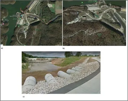
Fig.1.(a) Modeling area, Wappapello Lake, MO.U.S., (b) Spillway., (c) Upstream section.

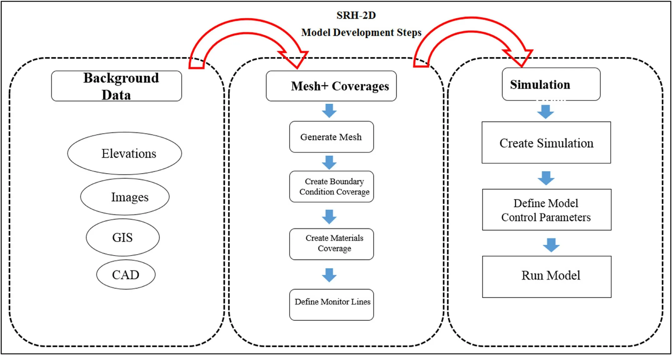
Fig.2.SRH-2D model development steps.

SRH-2D uses a flexible mesh that may contains arbitrar- ily shaped cells.In practice, the hybrid mesh of quadrilateral and triangular cells is recommended though purely quadrilat- eral or triangular elements may be used.A hybrid mesh may achieve the best compromise between solution accuracy and computing demand.SRH-2D adopts very robust and stable numerical schemes with a seamless wetting drying algorithm.SRH-2D is particularly useful for problems where 2D effects are important.Examples include flows with instream struc- tures, through bends, with perched rivers, with side channel and agricultural returns, and with braided channel systems.Fig.2 shows a step by step schematic of model development stages, based on SRH-2D, or the Sedimentation and River Hydraulics–Two-Dimensional model, for river systems under development at the Bureau of Reclamation.

2.3.2.GoverningEquations

Most open channel flows are relatively shallow and the effect of vertical motions is negligible.Thus, the most gen- eral flow equation (three-dimensional Navier-Stokes equa- tions) may be vertically averaged to obtain a set of depth- averaged two-dimensional equations, leading to the following well known 2D St.Venant equations:

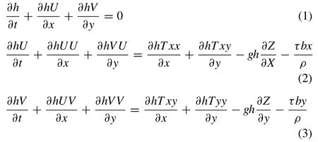
In above equations , t is time, x and y are horizontal Cartesian coordinates, h is water depth, U and V are depth- averaged velocity components in x and y directions, respec- tively, g is gravitational acceleration, Txx,Txy,Tyyare depth- averaged turbulent stresses, Zb, is bed elevation,ρis water density, andτbx,τbyare bed shear stresses (friction).

2.3.3.Discretization

The 2D depth-averaged equations in (1) to (3) may be written in tensor form as:

Boussinesq equations have been used to compute turbu- lence stresses:

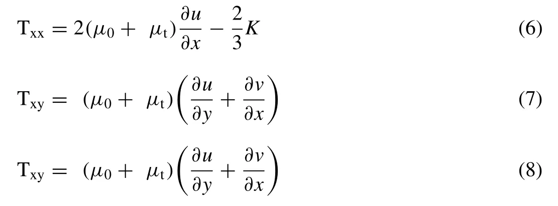
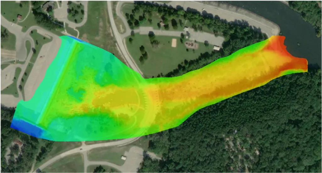
Fig.3.TIN from Scatter Data.

Whereis the mean velocity vector,is the 2nd-order tensor of turbulence stress with its component defined in Eq.(5) ,τbis the bed shear stress vector, andρis the fluid density [11] .U and v are the velocity components, z is the water surface elevation,μ0is the kinematic viscosity of the water,μtis the turbulent eddy viscosity and, k is the turbulent kinetic energy.Note that rainfall is omitted as it is used only for the diffusive wave equation.The governing equations are discretized using the finite-volume approach.The solution domain is covered with an unstructured mesh with each mesh element assuming arbitrarily shaped polygons.Most commonly used polygons are triangles and quadrilaterals.All dependent variables are stored at the geometric center of a polygon.The governing equations were integrated over a polygon using the Gauss theorem [12] .

2.3.4.Topographic-TINEditing

From 192940 individual bathymetric collected points (Scattered Data Points) raster and tin (Triangular-Irregular- Network) created and presented in Fig.3 [13]

Bed materials for upstream and downstream sides of the spillway are shown in Fig.4 a and b respectively.

2.3.5.Conceptualmodeldevelopment

Effective boundary was delineated and further divided into sub-areas to develop a conceptual model which are presented in Fig.5 [13]

Table 1 Manning’s Coefficient.

After boundaries delineation, the whole area divided into 6 zones based on the material types and roughness coefficients assigned to them.Zones 1 and 2 represent the main channel at the different sections.Boulders at the upstream side with higher roughness represents zone 1 materials.The extended part continued to downstream section consists of finer mate- rial with lower roughness represents zone 2.Left bank (zone 3) and right bank (zone 4) are the flood plain extension areas.Road connects the upstream and downstream sections (zone 5) and, finally top of the spillway (zone 6) which all shown in Fig.6 below [13–15] .

Table 1 shows the chosen roughness coefficients for dif- ferent zones (Supplementary Information)

2.3.6.MeshDevelopment

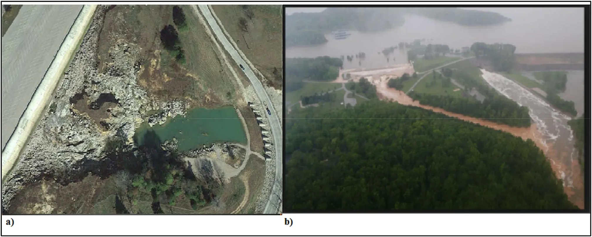
Fig.4.(a) Upstream (Cobbles and coarse gravel), (b) Downstream (Gravel and finer materials).

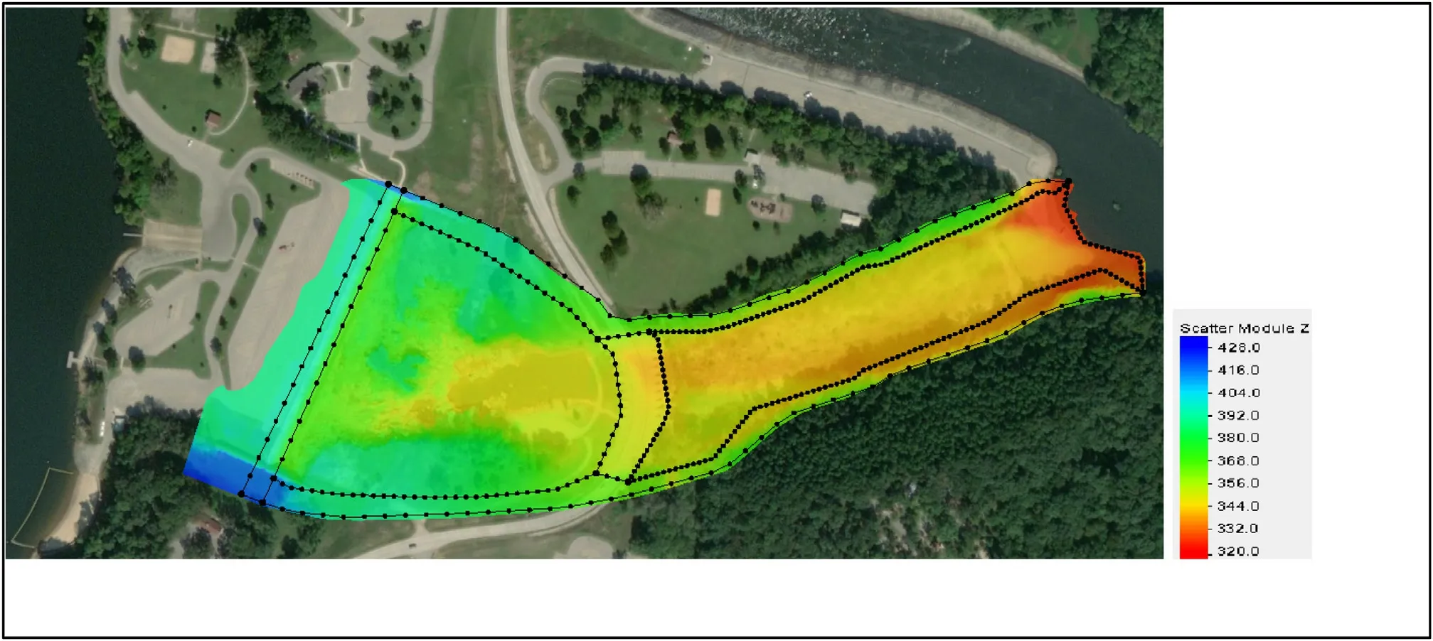
Fig.5.Boundaries delineation.

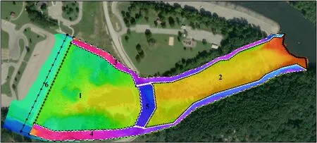
Fig.6.Material Zoning.

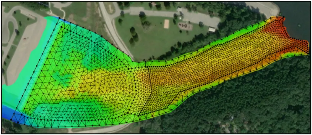
Fig.7.Different cell sizes attributed to sub areas Mesh assigned to different areas

When the delineation of different zones has been com- pleted mesh was assigned to the areas.Redistribution of the vertices has been done based on the grain size of the bed as well as separating flood plain boundaries.Paving bound- aries.Paving flood plain dboundaries separating flood pain boundaries separating the flood plain boundaries in compar- isonwith main channel paiving method was used in the mesh development procedure.Mesh sizes are smaller at the main channel in comparison tothe banks.Fig.7 shows different cell sizes which were attributed to subareas.Fig.8 shows the generic mesh which was created by applying map to 2D mesh command.with main channel mcain channel.Paving method was used in the mesh development procedure.Mesh sizes are smaller within the main channel in comparison to the banks.Mesh creation is based on the total area.Fig.7 shows different cell sizes which were attributed to different sub ar- eas.Fig.8 shows the generic mesh which was created by applying map to 2D Mesh Comands.[16] used in the mesh development procedure shows different cell sizes attributed to sub areasprocedure.Mesh sizes are smaller within the main- channel in comparison to the banks.Different xell sizes were attributed to sub areas.Mesh size are smaller within the main channel in comparison to the banks areas.Shows the differ- ent cell sizes attributed to the sub areas.Mesh creation is based on the total area.Fig.8 shows generic mesh which was created by applying map to 2D mesh command [16] Fig.8

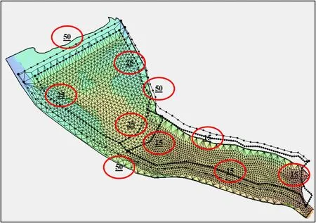
Fig.8.Mesh assigned to different areas.

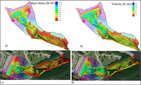
Fig.9.(a) Shear Stress 3D, (b) Flow Velocity 3D, (c) Shear Stress Plan View, (d) Flow Velocity Plan View.

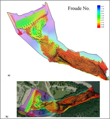
Fig.10.Froude Number for Steady State Condition (a) 3D, (b) Plan View.

Vertices were redistributed along each internal and exter- nal boundary as described below: All external boundaries considered to be 50 points, all the interior boundaries within the upstream side of the main channel considered to be 25 points, and 15 for the downstream of the main channel.excluding inflow and outflow lines These selective num- bers are the outcome of the combination of the conver- gence process with respect to time steps.There are two methods for generating the mesh.First is paving and the second is patching.Patching method uses rectangular el- ement which is much easier and faster in terms of the run time but paving approach uses triangular cells which means a bit longer calculations but more accurate re- sults.In this study paving method was applied to all the sub-areas.

2.4.Model Setup Information (boundary conditions, time steps, etc.)

In this part the modeling approaches and elements are de- scribed for both steady and unsteady State scenarios.Firstly, the boundary condition, were assigned, then SRH-2D simu- lation process and time steps were described.

2.4.1.AssigningBoundaryConditions

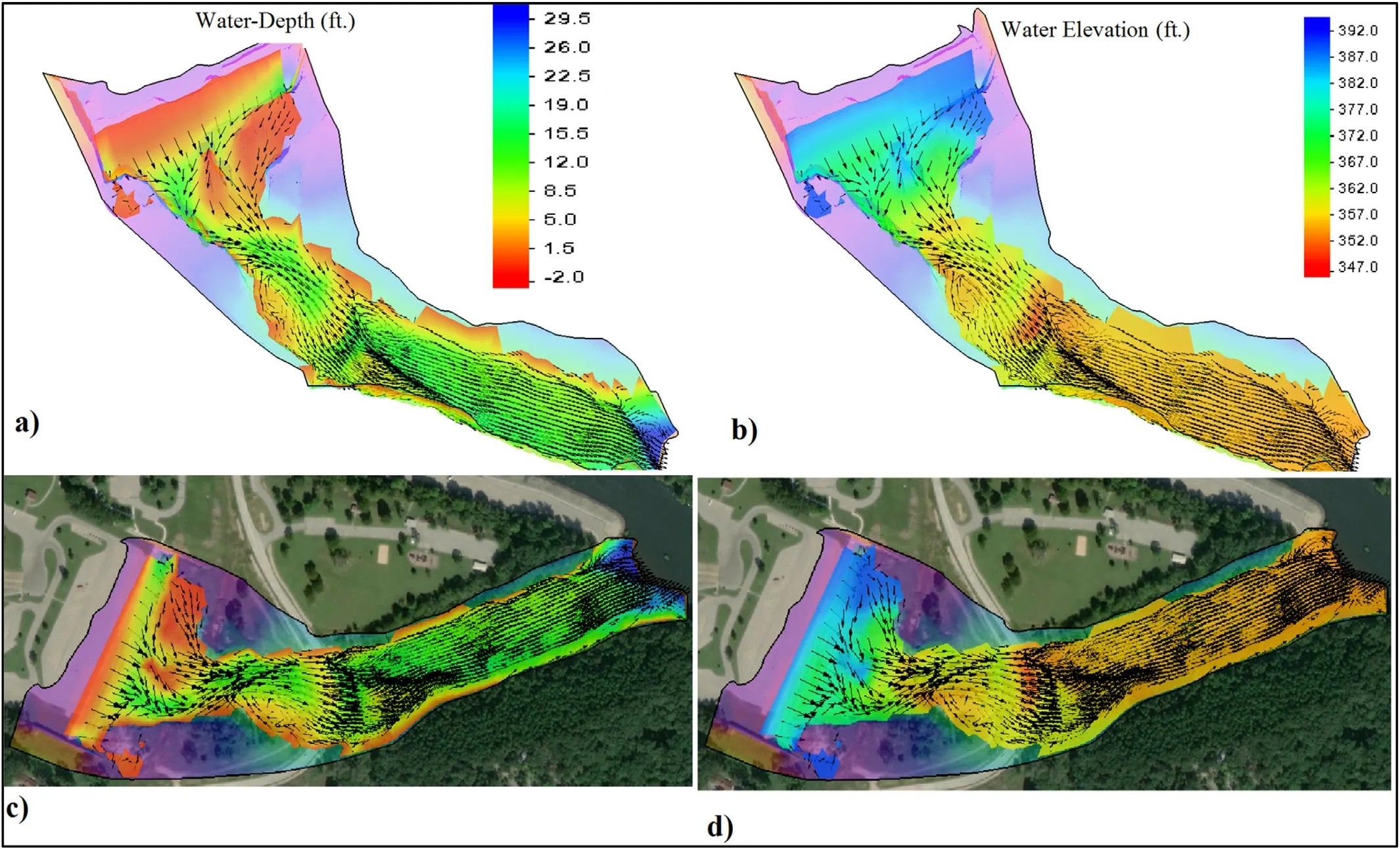
Fig.11.(a) Water Depth 3D, (b) Water Elevation 3D, (c) Water Depth Plan View, (d) Water Elevation Plan View.

Boundary conditions force certain hydrodynamic condi- tions to the model.For the steady state condition a uni- form discharge of 31000 cfs which has an approximately 25-yr return interval was assigned to the inflow.For un- steady flow condition a hydrograph for approximately 500–yr was applied.The downstream boundary condition for both Scenarios have been set to normal depth base on a rat- ing curve which mimics the situation.In the modeling ap- proach, a new coverage was created based on the initial domain and the model type has been set to SRH-2D bound- ary condition.Finally, inflow and outflow of both models were assigned.

2.4.2.DefiningtheSRH-2DSimulationandTimeSteps

The SRH-2D simulation was created as a separate entity in the SMS project.Different components for the simulation were associated (linked) to the simulation.Model parame- ters were assigned to the simulation.To create a new simula- tion all the needed coverages have been prepared in advance and properly linked to the model.Coverages such as domain, boundary conditions and materials were linked to both steady and unsteady model in the model controller before running the Simulation.Time step is one second and model ran for a period of 15 hours.

3.Results and Discussion

After completion of SRH-2D run, a XMDF file was gen- erated which has been called “Steady_XMDF.h5”.This file includes six sets of data as below: shear stress (Pounds per square ft.), Froude (dimensionless Froude number), Vel Mag (velocity magnitude in feet per second), Water_Depth_ft”: (depth of water in meters), Water_Elev_ft”: (water surface elevation in meters above the datum), Velocity”: (x and y components of velocity in ft per second).

3.1.Steady State Result

Fig.9 below shows the shear stress and flow velocity in lb./ft2and ft./sec respectively both in 3D and plan view.Shear stress variations are between zero to 12.6 lb./ ft2and the highest values are shown in blue which is the first location where free jet touches the ground from the top of the spillway.Accordingly flow velocity ranges from zero to 36.0 ft/sec.The highest flow velocity was assigned to the beginning of the upstream section where the free jet flow touches the ground [13] .Shear stress and flow velocity (Steady State Condition) are shown in Fig.9

Froude Number distribution which is ranged between zero to 4.5 at the green area which represents the spillway top and the very beginning of the upstream section where the flow condition is supercritical (Fr>1).The main part of down- stream section remains in the orange color zone which rep- resent the subcritical flow (Fr<1) and is almost below 0.9 ( Fig.10 )

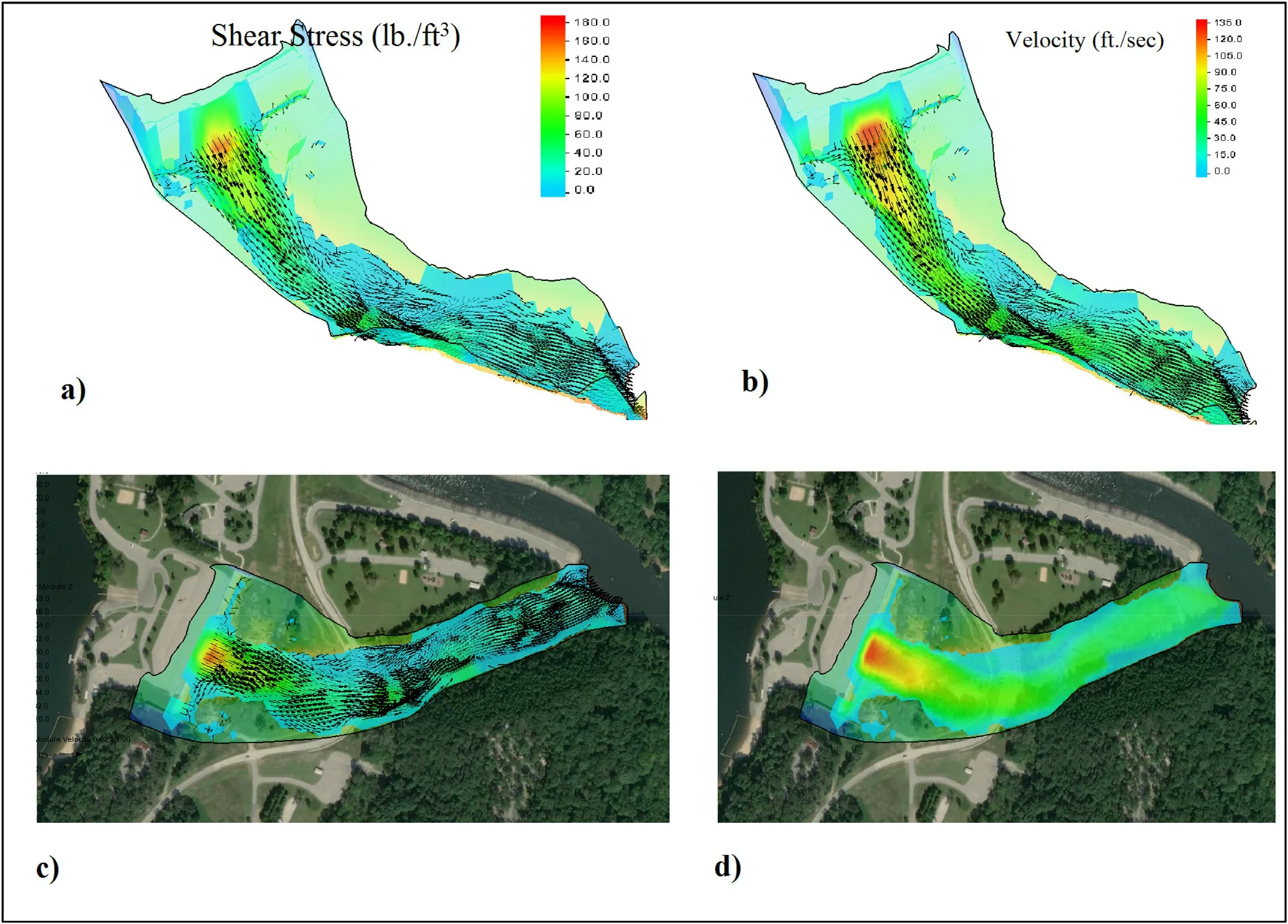
Fig.12.(a) Shear Stress 3D, (b) Flow Velocity 3D, (c) Shear Stress Plan View, (d) Flow Velocity Plan View.

Water depth and elevation ( Fig.11 ) have been presented in 3D and plan view [13] .Water depth starts with almost less than 1.5 feet at the top of the spillway.A thin sheet of fast flowing water which represents the supercritical flow condition at the upstream section of the channel continues to the downstream section where maximum depth possible occurs.(29.5 ft.) Here flow is completely tranquil indicating a subcritical flow condition.Water surface elevation is the sum of flow depth and datum for every single point.

3.2.Unsteady State Result

Shear stress and flow velocity in lb./ft2and ft./sec respec- tively both in 3D and plan view presented in Fig.12 .Shear stress variations are between zero to 180 lb./ ft2.The highest values are shown in orange which stands for the first loca- tion where free jet touches the ground from the top of the spillway.Shear is much higher in comparison to steady state flow condition.(160 lb./ft2 compare to 12.6 lb./ft2).The dif- ference shows turbulence effects of unsteady flow condition.Flow velocity ranges from zero to 135 ft./sec.The highest flow velocity was assigned to the beginning of the upstream section where the free jet flow touches the ground.(Orange area in figure 12 )

Water depth and elevation for unsteady flow condition ( Fig.13 ) were presented in 3D and plan view as well.Water depth starts with almost less than 2.35 feet at the top of the spillway.A thin sheet of fast flowing water which represents the super- critical flow condition at the upstream section of the channel continues to the downstream section where maximum depth possible occurs.(26.85 ft.) Here flow is completely tranquil indicating a subcritical flow condition (shown in dark blue).Water surface elevation is the sum of flow depth and datum for every single point.

Froude number for unsteady state flow condition ( Fig.14 ) shows a high range of variation due to turbulence flow con- dition starts with a value between 13.22 to 15.4 in dark red representing strong jump at the falling jet.Froude number de- creases as the flow moves downstream section which results in subcritical situation(Fr<1)

3.3.Erosion and Deposition Zone

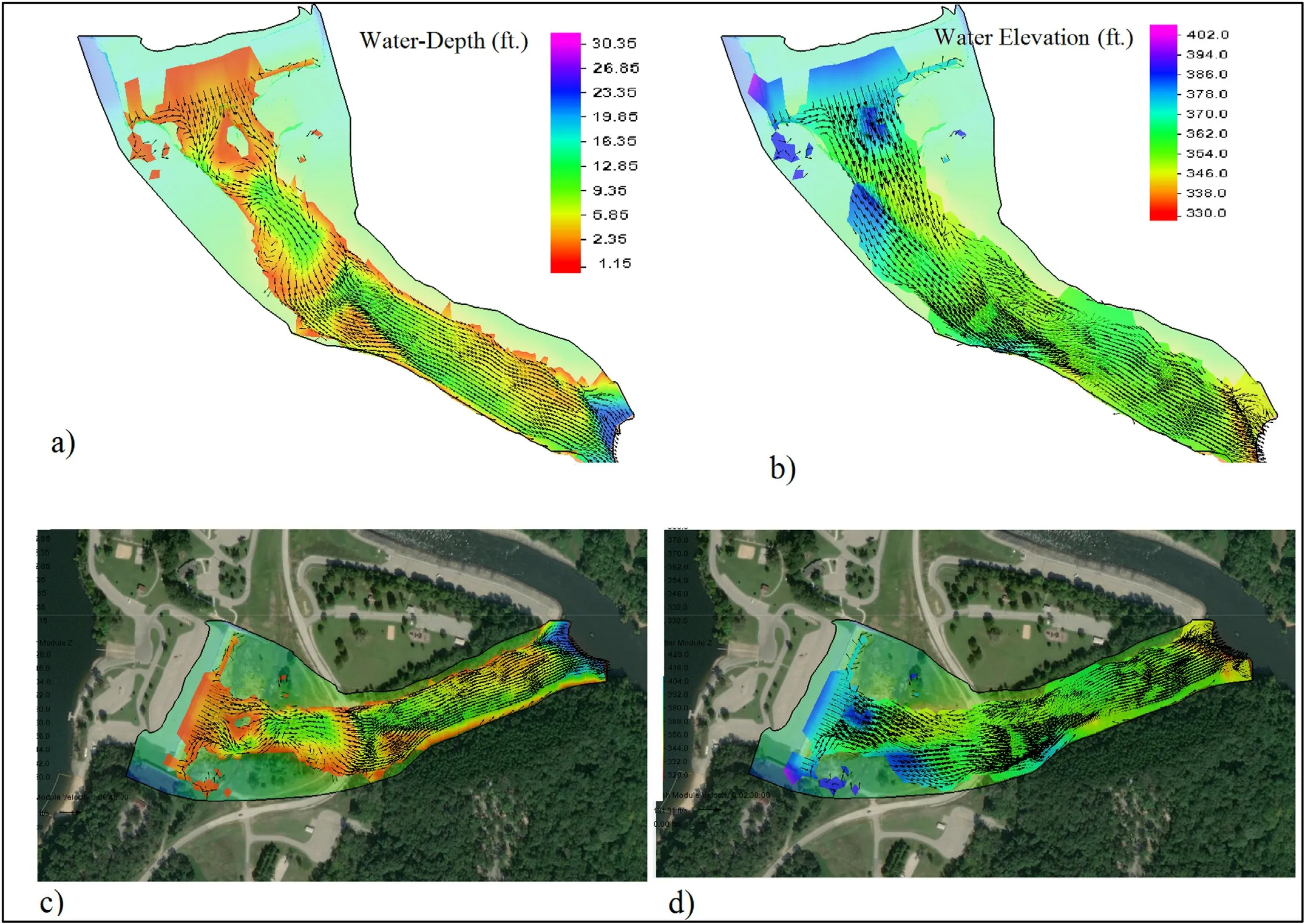
Fig.13.(a) Water Depth 3D, (b) Water Elevation 3D, (c) Water Depth Plan View, (d) Water Elevation Plan View.

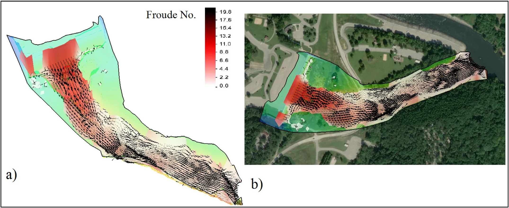
Fig.14.(a) Froude Number 3D, (b) Froude Number Plan View.

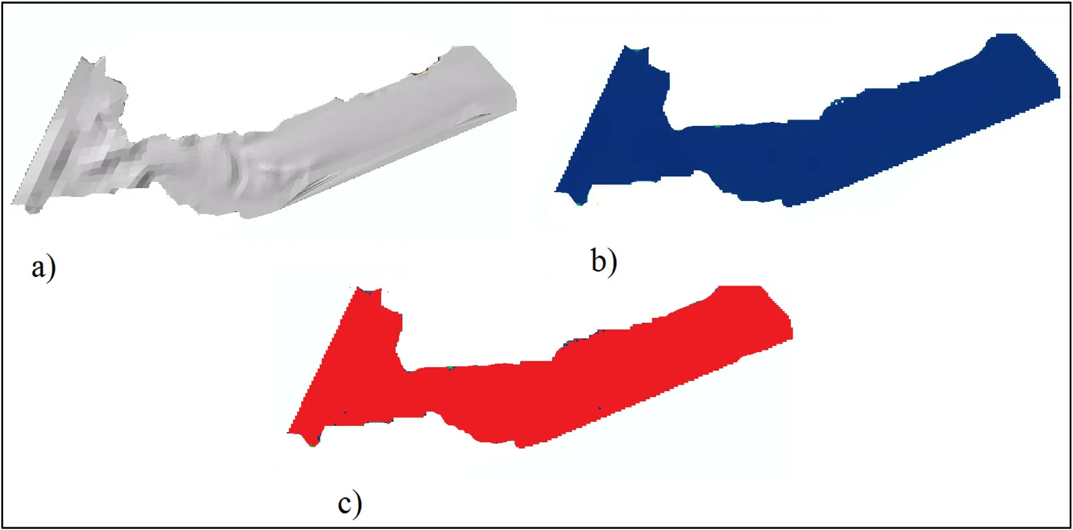
Fig.15.(a) Tin, (b) Raster, (c) Deposition areas, (Steady State Flow).

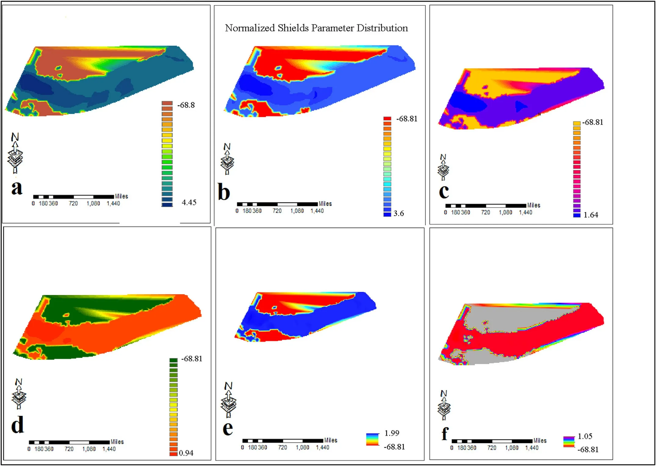
Fig.16.Normalized Shields Parameter Distribution, Time steps (a) to (f) (Unsteady State Flow).

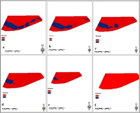
Fig.17.Deposition and Erosion Area, Time steps (a) to (f) (Unsteady State Flow).

Good estimation of erosion and deposition patterns re- quires a comparison between the critical shear stress (τ* ) with the critical shields parameter (τ?c).Wherever the ratio ofit represents the erosion and whenshows the deposition areas.Fig.15 shows three development stages of Normalized Shields parameter distribution for steady state flow condition, first based on the results of the shear stress, irregular triangular network (Tin) was created (15.a) then for further analysis tin was converted to a raster format (15.b) and, finally considering specific gravity of the particles, den- sity of fluid, grain average diameter and critical Shields pa- rameter a new raster file has been created to represent the deposition and erosion areas.As it is shown in (15.c) red areas are almost covered the flood domain which means at the steady state flow condition there is no concern regarding the erosion.New raster shows the deposition areas based on Normalized Shields parameter which created from the shear stress profile.For the steady state flow condition based on new raster ( Fig.15 c) red areas shows that the ratio is almost below one for entire area () which means there are no eroding areas but deposition.

The distribution of Normalized Shields parameters pre- sented in Fig.16 for different time steps of unsteady flow con- dition.The receding pattern of distribution is comprehended within simulation time which is presented within a to f.Sev- eral time steps of unsteady flow simulation presented from a to f (6 time steps) which presents the extension of Normal- ized Shields parameter with respect to shear stress from the maximum shear available to the minimum possible at the end of simulation period.As it is presented in figure 16 , first time step (a) which includes the maximum shear in the domain has the most extended Normalized Shields distribution.As the time passes it recedes through (a) to (f) and become smaller and smaller until the strength of shear stress almost dies out at the final stage (f).Based on the Normalized Shields dis- tribution the erosion and deposition patterns were calculated which is a good estimator of the areas prone to erosion and deposition.

In Fig.17 blue areas represent erosion which are mostly below the spillway and some parts of the downstream which contain the areas with higher velocities.Red areas represent the deposition which is a common process within the alluvial flow path.Based on Normalized Shields parameter distribu- tion a new raster layer was created which divides the entire area to erosion and deposition based onRatio ofrepresents the erosion and respectivelyshows the de- position areas.

Similar receding pattern of Normalized Shields parame- ter presented here and indicates that the erosion areas are the areas accompanied with the highest shear stress and flow velocities.As the flow moves towards tranquil situation the erosion areas getting smaller and smaller and, finally forms a tiny blue spot of erosion where exactly free jet collides the bed at upstream section.

4.Conclusion

Flow parameters such as Froude number, flow velocities.flow depth, shear stress in both steady and unsteady flow were investigated.Studying the Normalized Shields Parame- ter distribution ( Fig.16 ) in different stages of unsteady flow condition, illustrates erosion pattern within the main stream and nearby areas ( Fig.17 ) Similar kind of a thing happens in coastal areas when we do need to observe the sediment accumulation to reach sufficient anchorage depth for ships.This is a beneficial tool for annual or semi-annual dredging program in coastal areas.A comparison between the steady and unsteady states flow characteristics such as shear stress, flow velocity, Froude Number etc, have been done to have a better understanding of these parameters in both conditions and by the help of SMS SRH-2D the ranges of these variation presented in a graphical format.Normalized Shield parameter distribution calculated based on shear stress for both scenarios and the receding pattern was observed which was logical due to nature of the flow propagation during time-steps.Finally, deposition and erosion areas determined which could be use- ful indicator in terms of flood plain delineation as well as determination of dredging areas to provide a regular dredging program.

Declaration of Competing Interest

This work has been completely done by Farhad Sakhaeee and has no conflict of interest by others works.