?yvind ?ksnes Dalheim , Sverre Steen

a Department of Marine Technology, Norwegian University of Science and Technology (NTNU), Otto Nielsens vei 10, Trondheim 7491, Norway

b Rolls-Royce 1 University Technology Centre (UTC) – Ship performance and cyber-physical systems, Trondheim, Norway

Abstract Most applied time series are non-stationary, or exhibit some kind of non-stationarity for at least parts of the time series.For time series analyses or mathematical modeling purposes, the non-stationarities can be difficult to handle.Therefore, identification of stationary and non-stationary behavior is of great practical interest in time series analysis.In this study a robust and computationally efficient method to identify steady state parts of time series data is presented.The method is based on the class of deterministic trend models using a sliding window, and is focused towards being easy to implement, efficient and practical in use and to preserve data completeness.To demonstrate the performance of the steady state identifier, the method is applied on different sets of time series data from two ships equipped with systems for in-service monitoring.The method is shown to be reliable and practical for identifying steady state parts of time series data, and can serve as a practical preprocessing tool for time series data analysis.? 2020 Shanghai Jiaotong University.Published by Elsevier B.V.This is an open access article under the CC BY-NC-ND license.( http://creativecommons.org/licenses/by-nc-nd/4.0/ )

Keywords: Stationarity; Steady state; Signal extraction; Change point; In-service data; Ship monitoring.

1.Introduction

Inference of time series data often introduces the ques- tion of data stationarity.Whether the data is stationary or not defines how the data should be interpreted, and guides the selection of proper modeling tools and methods for doing the intended type of data analysis.Under the assumption of stationarity one can make inference based on a single realiza- tion.This is not the case if non-stationarities are present.For most practical applications, ensuring stationarity in time series processes is not achievable.This concerns particularly during long time span or in cases of environmental factors affecting the time series data [2] , as well as intermittent situations of human interference with the underlying process generating the time series data.The non-stationarities might occur in differ- ent ways; as time varying means, time varying variance or as a combination of these properties.In situations where some non-stationary behavior in the data is present, estimation of statistical parameters using a single realization while assum- ing stationarity of the process can lead to biased or inaccurate parameter estimates.If e.g.used to model physical behavior of a system at equilibrium, the non-stationary data violates one of the fundamental assumptions of the model.From this reasoning it follows that connecting the data modeling or an- alyzing procedures to the question of stationarity is necessary for unbiased interpretation of the data or model.In general, non-stationarity can be managed by either constructing mod- els that consider the time-dependent transient behavior, or by simply splitting the time series data into stationary intervals or windows from which the model parameters can be estimated.As models considering non-stationary behavior can become quite complex, identifying time intervals or windows suitable for stationary models is considered an important application in the field of data analysis.

Although many time series are non-stationary, parts of the time series can behave very similarly, e.g.in terms of variance or frequency content.The time series parts might however still differ in the local mean levels.[3 , p.85] refer to this kind of non-stationary behavior as homogeneous non- stationarity.A stationary part of a time series can, in many practical applications, be sufficient for data modeling using stationary models, provided that the duration of the station- ary part is sufficiently long.In order to identify changes in mean and variance of a time series, a first step is simply to visualize the time series plot.This is however most appropri- ate in case of a very limited amount of data.As the amount of data grows, it becomes unquestionably more desirable to employ computationally efficient techniques for identification of stationary time intervals.

The International Organization for Standardization (ISO) gives a recommended practice for evaluating ten-minutes blocks of data used to measure changes in hull and propeller performance of ships.The recommended practice is given in terms of threshold values for the standard error of the mean of rpm, speed through water, speed over ground and rudder angle [4] .The evaluated block of data is disregarded if one of the respective standard errors exceeds its limit, as a means to reveal unsteady behavior in the data.Experience with analysis of operational data from ships however shows that this steady state evaluation is somewhat too strict, particularly for ships experiencing large motions when sailing in waves.A fixed limit of the standard error of the mean of the ship speed is not optimal in case of analyzing ship behavior in waves, as large ship motions may cause significant variations in speed.The same argument holds for propeller rpm and for the rud- der angle, particularly when sailing in oblique waves.The method for steady data extraction is not very flexible, and has no distinction in the method that allows for adaption to the specific use of the steady data.There is a potential for improved data completeness as well as better control on the steady state identification that the recently developed method provides.

In statistics, the strongest form of stationarity is referred to asstrong,strictorcompletestationarity, for which thenth order distribution function is time invariant for any value ofn.A weaker form of a stationary process is referred to asnth orderweaklystationary, for which all of its joint mo- ments up to ordernexist and are time invariant [3 , p.8].That is, a second order weakly stationary process has con- stant mean and variance.Time series analysis often consider second order weakly stationarity, as the two first moments are relatively simple to check.For many practical applica- tions though, the requirements for a time series process to be stationary is even less strict, and for which the condition ofsteadystateis rather used.If the measured data is viewed as representing the true process value including noise and distur- bances, the steady state condition means that the true process value stays unchanged [5] .For the purpose of deterministic process modeling, the steady state condition does not require the associated noise and disturbances to be stationary.If how- ever further considerations regarding the stationarity of noise and disturbances are required, a steady state identification can perform weighted combined steady state identification of the true process value, the noise and the disturbances individu- ally rather than directly incorporating second order weakly stationarity.The same holds for practical applications where the state of a system is to be identified based on multiple process signals.

The problem of discovering incidents at which properties of time series data change is referred to as change-point de- tection.Various techniques have been developed for change- point detection, attracting a lot of attention particularly in the data mining community [6] .Among the studies facing this problem, a typical statistical formulation is to compare prob- ability distributions over two consecutive time intervals gener- ating the time series data, in search for a time point where the distributions become significantly different.Within this statis- tical framework, several approaches have been investigated.This includes techniques using generalized likelihood ratio estimation (GLR) and the cumulative sum control scheme (CUSUM), both which have been extensively explored in the data mining community.[2] developed a frequency domain test against non-stationarity in time series by comparing the goodness of fit in log-periodogram regression.The approach was built on a semi-parametric class of models, performing fairly good in detecting various non-stationary structures.For simply identifying intervals in a time series suitable for ap- plication of stationary models, the test is however somewhat complex to implement, as a proper basis functionψk( ·) that satisfiesmust be selected prior to applying the model.The cumulative sum control chart (CUSUM) is an- other widely used approach for change-point detection.The traditional approach is using a pre-specified mean shift to identify change-points, for which a satisfactory performance has been demonstrated.As the assumption of knowing the true mean shift prior to the application of the control chart can not always be met, [7] developed an adaptive CUSUM con- trol chart to detect a range of future expected and unknown mean shifts.[7] documented the performance of the one-sided control scheme only, and the authors remarked that the num- ber of parameters to be specified increases from two to four when adapting to the two-sided control scheme.For most practical purposes, a two-sided control scheme is necessary for constructing a robust change-point detector.Implement- ing this approach for change-point detection hence requires knowledge and experience in proper parameter selection, which can be found challenging for a number of potential users.

[6] proposed a non-parametric method for sequential change-point detection by estimation of probability den- sityratiosrather than the probability densities itself.As the parametric models rely on a strong model assumption, they tend to be less flexible in detecting change-points in real world data sets, which motivated the formulation of a direct density-ratio estimator.[6] confirmed that the pro- posed method could be an alternative to existing approaches for practical change-point detection.However, despite that the method avoids direct probability density estimation, six tuning parameters must be set, in addition to a predeter- mined fixed threshold value for the final decision of a change-point.

In parallel to the evaluation of probability distributions for change-point detection, a number of techniques using hypoth- esis testing have been developed to identify steady state of time series.[8] summarized previous work on steady state detection as either doing linear regression over a data win- dow with a subsequent t-test on the regression slope, using a t-test to compare two recently computed means, or performing an F-test on two recently computed standard deviations either from two adjacent windows or from the same window but us- ing two different filtered means.A method for online steady state identification using the F-test on the ratio of variances was developed by [5] , using two filtering factors to arrive at different estimates of the variance.Results agreed with vi- sual recognition of the system state, but the filtering nature of the identifier introduced a delay to the identification of steady state dependent on the filtering parameters and further conflicting with the amount of success of the identifier.[9] de- veloped a steady state detection algorithm using the t-test to determine if the difference between the process signal value minus its mean was above or below the standard deviation times its statistical critical value.The method assumed that the underlying system evolved with a non-zero slope multi- plied by its relative time within the window, i.e.a determin- istic drift component.The main contribution of [9] was to correct for the drift component when calculating the mean and standard deviation, leading to an unbiased probability es- timate of the stationarity of the process inside the window.There are however some shortcomings in using this method.If the length of the window is too short the process will not have time to stabilize, and the probability of stationarity will be low.If the length of the window is too long, multiple inter- vals of non-stationary behavior may in total form a stationary interval when in fact it is not.This is known as low/high frequency aliasing and under/over-sampling [9] .False indica- tions of stationarity may also take place in situations where the window is centered over a local peak of an oscillating process, giving a mean slope of the drift component equal to zero.

The interest in various time series data mining applications are continuously increasing, and so does the amount of real world generated sensor data [1] .With a greater amount of data becoming accessible for researchers comes an accompany- ing need for systematic and effective methods to extract only the most relevant data for a particular type of data analysis.Identification of steady state is highly relevant for most ap- plications of time series data, and tools specifically designed for this purpose might therefore contribute to more efficient implementations of time series data analyses.To overcome the shortcomings and complexity in state of the art meth- ods for stationarity detection, the present work demonstrates a practical and efficient technique to detect time intervals for which a continuous process exhibits stationary behavior in the mean, hereby referred to as steady state.Existing approaches require some user expertise to either define filters, parame- ters for probability estimation or tuning parameters.The new approach is therefore focused towards easy and practical im- plementation, being robust and computationally efficient as well as preserving data completeness by minimizing detec- tion of false negatives.The approach is based on hypothesis testing of the slope estimated from the time series data.Tra- ditionally, detection of steady state is applied in time blocks, which is suited for offline steady state detection.The present technique is implemented in a time shifted approach using a sliding window, which is mostly seen in real-time implemen- tations.A sliding window requires several more calculations compared to using blocks with no overlap.For most steady state detection problems however, the computational burden is not expected to be of any practical significance, and the potential increase in computational burden is balanced by the improved performance in terms of preserving data complete- ness compared to using a traditional block evaluation.

2.Method

In this study, a time series model is applied to perform offline steady state detection on time series data gathered from the in-service monitoring systems installed on a gen- eral cargo/multipurpose vessel (MPV) and a platform supply vessel (PSV).The MPV is mainly carrying cargo along the Norwegian coast, while the PSV is mainly serving offshore platforms in the North Sea.The two monitoring systems col- lect data from sensors installed on a wide range of equipment onboard the ships, sampled at a frequency of 1Hz.In this study, a selection of sensor variables is chosen based on dif- ferent interpretations of steady state behavior, which will be presented and discussed.The method is developed for offline steady state detection.However, due to the nature of the used techniques, the method can be used for online steady state detection as well.

2.1.Mathematical approach

For any of the process signals, the fundamental assumption about the behavior of the underlying system is that it can be modeled by a deterministic linear trend model regardless of the window selection.The model is expressed as

withatbeing a zero mean white noise process with constant variance,b0being the intercept of the linear model andb1tthe linear deterministic drift component formed by the slopeb1and the relative timetwithin the window.Subscripttis a time index noting the time instant that the sample represents inside a window, starting fromt= 0 for all windows.The model in (1) is the simplest type of a process modeling non- stationary behavior in the mean.

The linear slopeb1is estimated by ordinary least squares estimation as

withnbeing the number of sampled values ofztin the window.The process is non-stationary in the mean if there is detectable accumulation in the signal, modelled by the slopeb1.

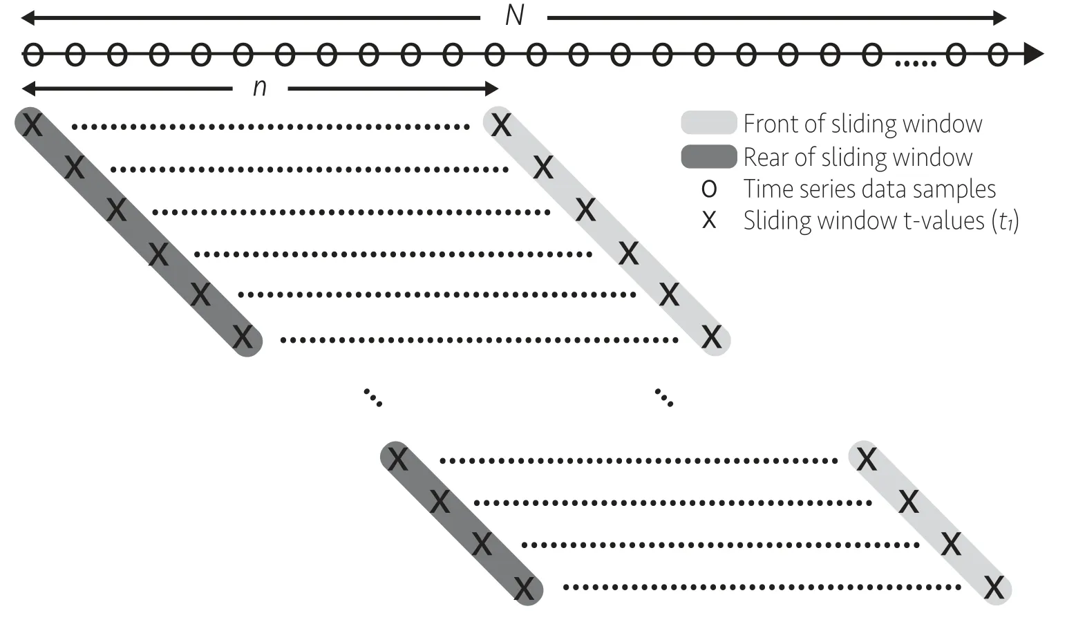
Fig.1.Illustration of time series data samples (circular markers) and the sliding window t -values (cross markers), where the light grey color encircles the front of the sliding window and the dark grey color encircles the rear of the sliding window.The two sets of t -values forms the steady and unsteady change point detector.

An estimate of the interceptb0is found by subtracting the estimated linear drift componenttfromzt:

By having an estimate of the drift slope and the intercept, the white noise standard deviation can be estimated from:

and hence the standard deviation ( ?σb1) of the estimated slope:

Under the assumption of independent normal innovationsat, the null-hypothesis that the process signal is stationary about the window sample intercept (b0) can be tested.A two- tailed t-test on,using thet-value from (6) , is applied to test whether the slope is significantly different from zero, indi- cating non-stationary behavior.The null-hypothesis is rejected for |t1|>tα/2,n?2(the criticalt-value) wheretα/2,n?2follows a Student’st-distribution that depends on the significance levelαand the degrees of freedomn?2.The value oftα/2,n?2for a specifiedαandncan be found using tabulated values of the Student’st-distribution or by using built in functions such as the Matlab functiontinv(p,nu), wherep= 1 ?α/2 andnu=n?2.Interpreting whatissignificant needs however to be discussed for the particular application of the steady state detector.Rejecting the null-hypothesis means that the state of the window is flagged as unsteady (st= 0), while a support of the null-hypothesis is flagged as steady state (st= 1 ).

The probability of the process being stationary over the window must be computed based on the test statistics.Be- cause the windows are overlapping,N+ 1 ?nnumber of sig- nificance tests are performed, withNbeing the total number of samples in the series andnthe number of samples in the moving window.For simplicity the windows have maximum overlap, i.e.the propagation of the window is a single unit of the time indext.Except for at the process signal ends (start and stop) there areksignificance tests of the estimated sig- nal slope in the window that represents each sample, withkbeing equal to the window sizen.Towards the process signal ends,kare truncated with unity for each sample, andk= 1 fort= 1 andt=N.

The simplest form of the steady state probability estimate is the arithmetic average of the test statistics output (st) over theknumber of test results for each sample of the time se- ries.The arithmetic average ofstforms the amount of the windows, containing the particular data sample point, that is identified as steady state.For final evaluation of the state of the sample point, a threshold value at which the sample is considered to be at steady state is needed.All windows con- taining the particular sample have equal contribution to the steady state indicator, however, a weighting of the windows can also be added.

A more delicate steady state identifier is developed to fully utilize the features of the sliding window.The identifier is built on the principle of a change point detector, that search for time points at which the properties of the estimated slope test statistics change.For each window, the test statisticst1is written to a matrix that is structured according to Fig.1 .

The cross markers in the figure illustrates the positions in the matrix to whicht1is written for each window.All other fields remain empty.The shaded areas in light and dark grey marks the position of the front and rear samples of the sliding window, respectively, which are used as the change point indi- cators.A change point is detected each time the test statistics exceeds or gets below the criticalt-value, determined by the significance levelαand the window sizen.The front samples reacts on the change of state from steady to unsteady, while the rear samples reacts on the change in state from unsteady to steady.

The time series data is processed with a moving win- dow using overlap, which more or less enables a straight- forward adaption to real-time applications.A new calcula- tion of steady state is run as each new sample arrives.A change in the state from steady to unsteady can be detected in real-time, however, a change in the state from unsteady to steady will have a time delay equal to the size of the sliding window.

2.2.Setting the parameters

The steady state detector has two parameters that must be set; significance levelαand window lengthn.The signif- icance levelαrepresents the probability of a type I error, or the probability of rejecting a zero slope (b1= 0) when a zero slope in fact is true.The window lengthnis mea- sured in number of samples, rather than in units of time, and must therefore be seen in relation to the sampling fre- quency.When adjusting the two parameters, the application of the steady state time series data must be considered.Using a filter analogy, the purpose of the steady state detector is to filter out undesirable effects from the time series data.The filter should however not only remove parts of the frequency content, as is for a high-, low- or bandpass filter, but rather detect intervals of the time series data that can be flagged as steady state according to the application of the data.The choice of window lengthnmust therefore be related to the effects we want to remove from the data.Using a long win- dow, unsteady behavior with short duration is hard to detect.On the other hand, a long window is well suited for detecting a typical sensor drift causing the sensor value to accumulate with time.A short window is more likely to let such a sensor drift pass the steady state detection, but will on the other hand be well suited for detecting unsteady behavior with short du- ration.In general, the window length must be longer than the autocorrelation persistence of known system dynamics that are acceptable even for a condition of steady state, but short enough to detect undesirable changes in the process value that has short duration.

The significance levelαcontrols the accepted slope in the steady state data.As a stand-alone parameter, it is related to the importance of a process value being at steady state when doing data analysis or mathematical modeling founded on the steady state assumption.If steady state in a process value is critical for the application of the time series data, the steady state detection must ensure a low probability of a type II error, or the probability of accepting a zero slope (b1= 0) when a non-zero slope in fact is true.This is equivalent with allowing for a high probability of a type I error, which is accomplished by using a higherα.This will increase the reliability in the steady state data, but on the other hand reject large parts of the data set, which is unfavorable for data completeness.Similarly, the less critical variables should accept a higher slope in the data window, which means accepting a higher probability of a type II error.Accepting higher probability of a type II error means using a lowerα.

Another consideration regarding the choice of parameters relates to using the window length to adjust the disposition to accept partly unsteady data in the steady state time series data.As a result of the sliding window, a longer window means that the state of the process in a longer run before and after the sample at study contributes to the overall probability of the local steady state.The result can be that it will take some time for the state to be flagged as steady, causing the overall amount of false rejections of the null hypothesis to increase.The resulting steady state data set will on the other hand consist of data that has reached a steady state condition for a period of time both prior to and after the detected steady state interval.

2.3.Interpreting steady state in ship data

When considering steady state operation of a ship, it is essential to interpret what steady behavior of a process means in terms of its physical system as well as the aim of the data analysis.We can refer to this as identifying thecriticalvariables for what we aim to study using steady state models.

A first consideration is to identify data sampled under a constant command of the ship.That is, time intervals at which control variables such as the propeller rotational speed (rpm), engine power or ship heading are kept constant.Constant command is mostly required for all kinds of steady state models.In other situations one might also require constant environmental conditions, in terms of a constant sea state, av- erage wind speed and direction, or a constant ocean current.When doing a performance analysis of a ship, it is important to ensure that data sampled under acceleration or decelera- tion of the ship speed is excluded, as well as time intervals when the ship performs a maneuver or is simply changing its course.The critical variables are hence the propeller rpm, engine power or propeller shaft power as well as the ship heading.If the interest is in the relation between waves and ship motions or if the data is used for shipboard sea state estimation, the ship speed in addition to the ship heading are the critical variables.Additionally comes the variables defining the wave environment itself, which should be fairly constant.

Interpretation of steady state for a ship deals with the ques- tion of how to separate ship commands from external impact of wind and waves - to filter natural dynamics from ordered changes.This relates to both the choice of critical variables as well as how large variations that can be accepted before the time series is marked unsteady.

Fig.2.Time series of propeller rpm data used as test case for steady state identification.

3.Results

To demonstrate the steady state detector, a selection of time series data from two ships is used.First, a demonstration of steady state identification on a standalone variable is shown.The selection of signal follows the interpretation of steady state for a ship, as discussed in Section 2.3 .The first applica- tion of monitored ship data relates to a performance analysis, and hence one of the critical variables for detection of steady state is the propulsion control signal.For the particular ship used for this demonstration, the propulsion control signal is identified from the propeller rotational speed (rpm), measured on the propeller shaft.Fig.2 shows a time series of 5 hours propeller rpm data used as a case for the steady state identi- fication.The time series case includes different levels of the propeller rpm, some short but rather abrupt changes as well as some small adjustments, all which are interesting to test on a steady state detector.First, results of steady state detec- tion using a state of art implementation with fixed window is shown, followed by a basic implementation of a sliding win- dow using the arithmetic average of the test statistics.Then, the performance of the new steady state detection approach using the front and rear values of the sliding window test statistics is presented and evaluated against the two first ap- proaches.The new approach is further evaluated using time series data from other signals.In the end follows a discus- sion on how to perform steady state detection when the data analysis depends on multiple critical variables.

3.1.State of art, stepping window

A steady state detection is applied on the propeller rpm data using the approach of [9] .The method is a stepped win- dow algorithm that runs an individual t-test on each sample in a window to check if the sample is inside a chosen con- fidence interval around the mean of the time series window.The confidence interval is a function of the window lengthn, the significance levelαand the unbiased estimate of the standard deviation of the process noice.In this example, a window with lengthn= 300 (5 minutes) is used for the rpm data, and the significance level is set toα= 5% .The window length is set to enable detection of changes having short dura- tion, since the rpm in this case closely resembles the control signal for the propulsion.The value ofα= 5% is set because steady state in the propeller rpm is not extremely critical for this particular case, so a 5% probability of incorrectly reject- ing steady state is accepted.A performance analysis usually average the data over some minutes, so small adjustments of the propeller rpm can be accepted.

The third parameter that must be set is the threshold value for a window to be steady when all the samples inside the window are evaluated according to the test statistics.The pa- rameter is a measure of the fraction of samples inside the window that is flagged as steady, or a measure ofhowsteady the window in total is.In this case it is set to 90%, which means that 90 out of 100 samples in the window must fulfill the requirement for being steady in order to flag the window as steady.

Results are shown in Fig.3 , with the colour indicating the state for each sample, red for unsteady and green for steady state.In Fig.3 a the first window runs from the first sample in the time series data.In Fig.3 b the starting point of the first window is shifted 30 samples relative to the first sample in the time series data.In both cases, several of the identified steady state regions agree with visual identification.However, depending on the starting point of the first window, the ap- proach also detects parts of the times series data at steady state even though this is clearly not the case (false positives).The first example of this is the major drop in propeller rpm when approaching 30 minutes into the time series.When the first window is shifted 30 samples relative to the first sam- ple in the time series, the approach identifies this drop as a region of steady state.The reason for this is that one of the windows becomes centered over the rpm drop, giving an es- timated slope in the window not significantly different from zero.Two similar situations occur around 180 minutes and 330 minutes into the time series where the propeller rpm has two clear drops.However, in these two situations the drops are identified as steady state for both of the two window starting points.Increasing the threshold for the steady state fraction from 90% to 95% gives a considerable lower amount of steady state, however has no influence on the problem of obvious false positives.Such behavior must be expected using this approach, and care should be taken when interpreting the results.In Fig.4 , a detailed view from the part of the time series around time [min] = 30 that is incorrectly detected as steady state is shown to the left.To the right in the figure, the same part of time series data is shown in a performance plot (performance being measured as the consumed shaft power vs ship speed).In this example, the deviation between the low performance and the high performance for the same ship speed is almost 40 percentage points, or in other words, the low performance is off by almost five times the high per- formance value.Including this part in the steady state data would mean a considerable influence on the overall perfor- mance evaluation of the vessel.So, even though the method performs well in detecting regions of steady state behavior where this really is true, the method will often fail to reject parts of the time series as steady state that certainly not is the case.The presented example of steady state detection shows how the method is sensitive to the starting point of the first window, and how the resulting steady state parts of the time series, and by that the performance evaluation of the ship, depends on this.

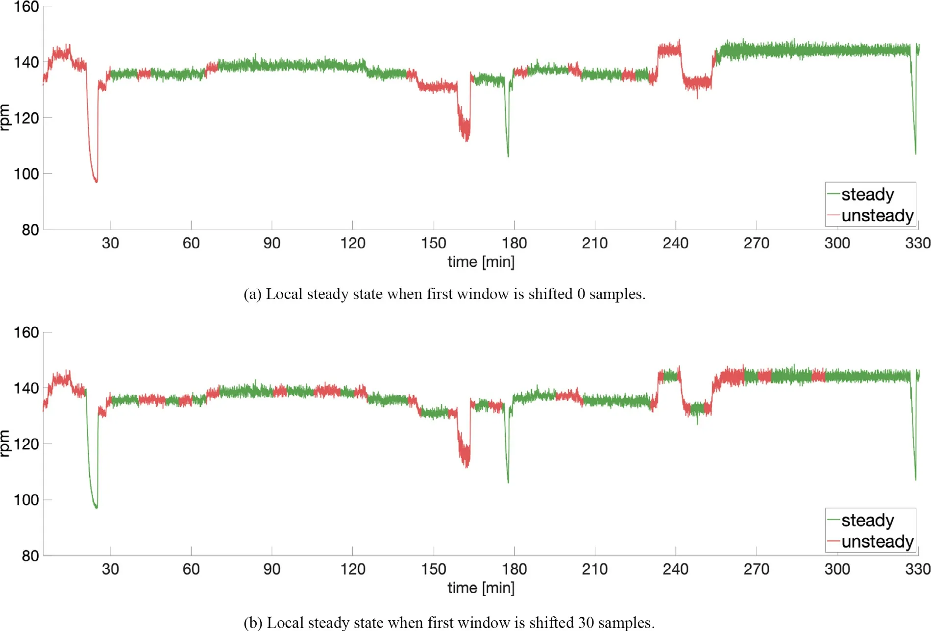
Fig.3.Time series of propeller rpm data showing local steady state using a fixed window of size n = 300 (5 minutes) with two different starting points for the first window.The significance level is α = 5% .The criteria for the data inside the window to be steady is that more than 90% of the samples within the window is identified as samples at steady state.

Fig.4.Detailed view from part of propeller rpm time series that is incorrectly detected as a steady state interval using stepped window.Plot to the left shows the time series data, where dark grey color with triangular marker facing down indicates part of time series where the rpm is decreased.Light grey color with triangular marker facing up indicates part of time series where the rpm is increased or approaching a steady value.The plot to the right shows the same part of time series data in a performance plot, with identical markers and colors.If this part of the time series was detected as steady state, the performance of the ship (measured as the consumed shaft power vs ship speed) could be off by almost five times the true value.

Fig.5.Time series of propeller rpm data showing local probability of steady state by taking the arithmetic average of the calculated state ( s t ) based on the t?test statistics ( α = 5% ).Model with sliding window.

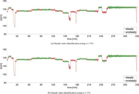
Fig.6.Time series of propeller rpm data showing local steady state identified using the new approach with a sliding window of size n = 300 (5 minutes).Two different significance levels are used for the t -test of the estimated slope.

3.2.Sliding window, arithmetic average of test statistics

In Fig.5 , results from steady state detection on the pro- peller rpm data using a t-test on the slope is shown.A sliding window withn= 300 (5 minutes) is used, and the method evaluates the arithmetic average of the calculated state (st) based on the test statistics.The color indicates the local steady state probability estimate for each sample, going from red as themostunsteadyto green as themoststeady.The rpm data in each window is tested for a nonzero slope us- ing the same significance level as for testing the individual samples in the stepping window approach (α= 5% ).The ap- proach identifies regions where the propeller rpm probably is at steady state.Such a region is seen towards the end of the time series, which also agrees with a visual identification of steady state behavior.The approach also correctly rejects the most evident unsteady parts, by assigning a very low proba- bility of steady state (P<0.1).Because the window is slid- ing with maximum overlap, the rejection is also found to be independent of the starting point of the first window.How- ever, a clear drawback is that further evaluation of the steady state time intervals depends on a threshold value set for the local probability, which for practical purposes can be difficult to determine.This is similar as for the method with stepping window presented in Section 3.1 , where the required fraction of steady state samples in a window had to be set.Without a threshold, the steady state detector only gives the most prob- able steady state samples rather than the actual time intervals of steady state data.

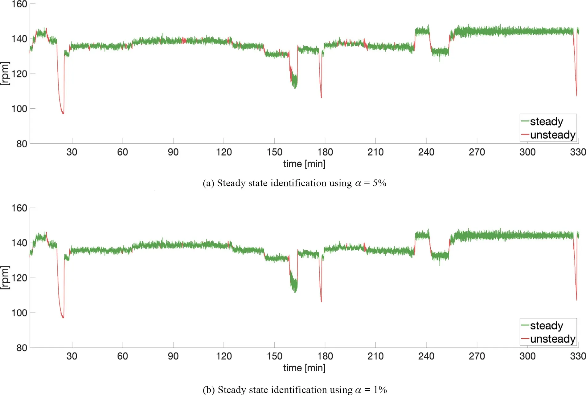
Fig.7.Time series of propeller rpm data showing local steady state identified using the new approach with a sliding window of size n = 60 (1 minute).Two different significance levels are used for the t -test of the estimated slope.

3.3.Sliding window, new approach

In Fig.6 , results from steady state detection on the pro- peller rpm data using the new approach with a sliding win- dow (n= 300) is shown, with two different significance lev- elsα= 5% andα= 1% .The color indicates the local state identification, evaluated using the front and rear collection oft-values as change point indicators.The approach identifies regions where the propeller rpm probably is at steady state, shown with green color in Fig.6 , and with respect to the detected states there are only minor differences between the two significance levels.A region of steady state is partic- ularly seen towards the end of the time series, which also agrees with a visual identification of steady state behavior, and the result from the application of the two previous meth- ods.The method successfully rejects parts of the time series that clearly not is at steady state, for instance the drop in propeller rpm at 15, 25, 160, 180 and 330 minutes, and the change in mean propeller rpm seen at 70, 125, 140, 205, 235, 245 and 255 minutes into the time series.All of these propeller rpm changes are detected for both of the chosen significance levels.Due to the sliding window the rejection is also independent of the starting point of the first window, which was identified as one of the critical drawbacks using the state of the art method with stepping window.However, the method also rejects parts of the time series that one by visual identification could expect to be at steady state, for example the part around 120 minutes into the time series.This may be due to the size of the window, or it could be due to the time series part in fact being unsteady.By us- ing a smaller window size, the detector is allowed to mark smaller parts of the time series as steady.The drawback is however that drift in the signal is more likely to be accepted.In Fig.7 , steady state detection is shown using a 1 minute (n= 60) sliding window.Decreasing the length of the win- dow gives a steady state detection that preserves more of the data as steady state, while the clear unsteady behavior of the rpm data where the level of the propeller rpm is changed still is flagged as unsteady.This is also the case if the starting point of the first window is shifted, because the method is not sensitive to where in the time series data the steady state detection starts.If we compare Fig.6 a and 6 b, it is shown how a lowerαpreserves more of the time series as steady.

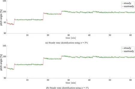
Fig.8.Time series of propeller pitch [%] data showing local steady state identified using the new approach with a sliding window of size n = 30 (30 seconds).Two different significance levels are used for the t -test of the estimated slope.

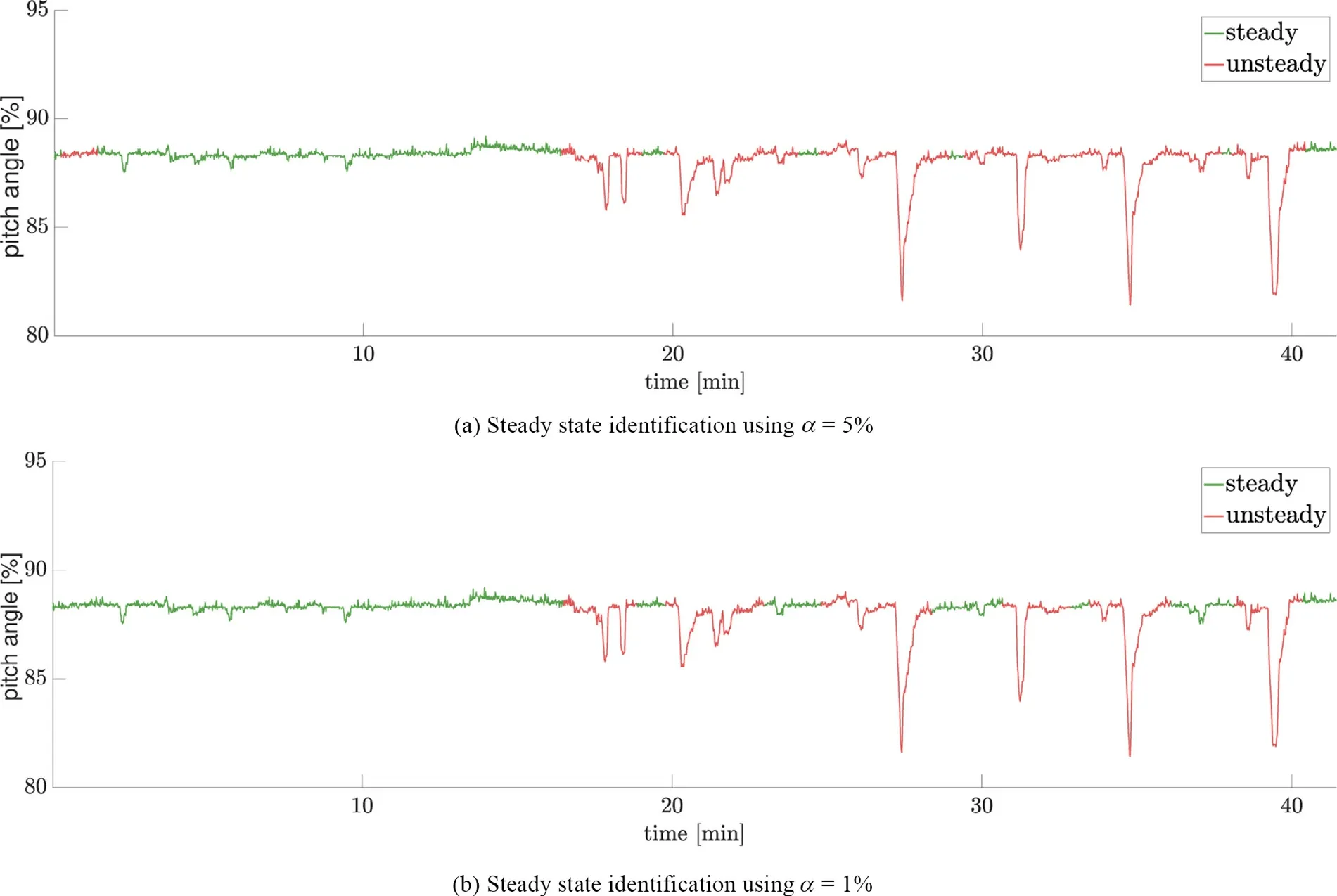
Fig.9.Time series of propeller pitch [%] data showing local steady state identified using the new approach with a sliding window of size n = 30 (30 seconds).Two different significance levels are used for the t -test of the estimated slope.

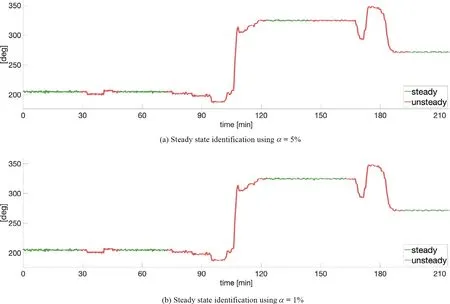
Fig.10.Time series of ship heading data showing local steady state identified using the new approach with a sliding window of size n = 1200 (20 minutes).Two different significance levels are used for the t -test of the estimated slope.

The detector accepts a higher estimated slope inside the win- dow, while the clear regions of changing propeller rpm level still are flagged as unsteady.

If the ship is equipped with a controllable pitch propeller, identification of steady propeller pitch is of similar importance as of propeller rpm with regard to a performance analysis of the ship.Both the propeller rpm and pitch are adjusted when controlling the forward speed.However, the rate at which the propeller rpm and pitch angle are adjusted relative to each other, depends on the configuration of the propulsion control system.Time varying propeller pitch relates to unsteady op- eration of the ship, for which transient effects may affect the performance analysis.In Figs.8 and 9 , two time series ex- amples of steady state identification on propeller pitch data from the multipurpose cargo ship is shown.Both examples show steady state identification using two significance levels (5% and 1%).The first example ( Fig.8 ) shows part of a time series where the propeller pitch is stepwise increased towards 100%.Each step is flagged as unsteady by the new method to identify steady state, regardless of the two significance lev- els, which only has minor influence on the final result.The second example ( Fig.9 ) shows part of a time series where the propeller pitch has more frequent and abrupt changes.Ev- ery large drop and rebuild is flagged as unsteady, regardless of the two significance levels.Both of the two examples of steady state identification on the propeller pitch time series data appears reasonable according to a visual identification, and the new steady state identification method demonstrates a reliable performance for a variety of unsteady behavior.

So far, steady state identification on variables critical for a ship performance analysis has been evaluated.There are however vast objectives for analyzing ship in-service moni- toring data.To further demonstrate the use and performance of the new method, steady state identification on ship data that may be used for other applications is also presented.The examples use time series data of measured ship heading and ship speed over ground (SOG) from a PSV to check for time intervals when the heading and when the ship speed is steady.Steady ship heading and speed data is by instance necessary for a wave - ship motions analysis, or to shipboard sea state estimation.The steady state identification is performed indi- vidually for each of the time series, and the results are shown in Figs.10 and 11 for ship heading data and ship speed data, respectively.In a traditional wave - ship motion analysis or for shipboard sea state estimation, a window size of 20 min- utes is typically recommended in order to obtain statistical independence from the particular realization of the wave en- vironment.Hence, a sliding window of sizen= 1200 (20 minutes) is used.

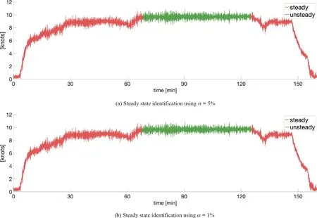
Fig.11.Time series of ship speed over ground (SOG) data showing local steady state identified using the new approach with a sliding window of size n = 1200 (20 minutes).Two different significance levels are used for the t -test of the estimated slope.

The identification of steady state in the ship heading data, shown in Fig.10 , has good agreement with visual identifi- cation.The effects of decreasing the significance value fromα= 5% toα= 1% are small, and the only change of any par- ticular importance is the increased length of the steady state time interval between time = 120 and time = 165 [minutes].Short intervals of apparently steady state data have been re- jected due to non-sufficient length compared to the window size.The method also successfully rejects small but distinct changes in heading as steady state, as by example shown at time = 30 [minutes].

3.4.Combined steady state identification

The new approach for steady state identification has shown good performance on standalone critical variables.For other time series data analysis purposes, steady state can be required for multiple variables at the same time.The procedure to combine steady state identification when having more than one single critical variable is to perform standalone steady state identification on all critical variables, and combining the steady state time intervals to form a final set of time intervals where all critical variables meet their steady state criteria.

In other cases, a more strict sense of stationarity can be re- quired, as for example second order weak stationarity where the process should fulfill both constant mean and variance.Going from steady state to a higher order of stationarity more or less follows the same way of combining steady state time intervals.However, the various moments of the critical vari- able up to the preferred order of stationarity must be calcu- lated prior to the steady state identification.If second order weak stationarity of a critical variable is preferred, the steady state time intervals of the mean and the steady state time intervals of the variance are combined to a final set of sec- ond order weak stationary time series intervals.Similar is for higher order weak stationarity.

4.Conclusion

The new method for steady state identification of time se- ries data is based on using a sliding window and its corre- spondingt-value of the local slope as a change point indica- tor.Through a number of demonstrations the new method is shown to perform well on a diverse selection of measurement variables collected onboard two different case vessels.The main advantage of the new approach relative to state of art methods is that it is very robust against false identifications of local steady state.That is, it ensures that the identified state is completely independent of the starting point of the first win- dow used for evaluating the state.Secondly, the new method only requires two parameters to be set by the user.These pa- rameters have clear physical meaning, which means that the user can interpret and specify the parameters relatively easily.

The main drawback of the new method is that it involves several more calculations compared to state of art methods.Yet, for most practical purposes it is found to be computation- ally efficient, as long as the steady state identification does not have to consider a large number of variables at the same time.Secondly, the new method does not consider a strict sense of stationarity, which means that it should only be used with the objective of detecting a weak sense of stationarity in terms of mean and/or variance.

Compared to a simple arithmetic average of the evaluated state of each sample, the new method is practical in both implementation and interpretation.This is much due to the fact that it is not depending on a threshold value for the local steady state probability.The new method is shown to manage variations in the signal variance, variations in the duration of the changes in the process value as well as the length of the typical steady state parts.The conclusion is therefore that the new method for steady state identification is a practical, robust and easy-to-implement preprocessing tool for time series data analysis.

Declaration of Competing Interest

The authors declare that they do not have any financial or nonfinancial conflict of interests.

Acknowledgement

The research presented in this paper was financed by Rolls- Royce Marine AS1and carried out as part of the Rolls-Royce1Kongsberg Maritime AS since April 1st 2019 University Technology Centre (UTC) at the Norwegian Uni- versity of Science and Technology in Trondheim.The authors gratefully acknowledge Rolls-Royce Marine AS for providing the full-scale data used in the research.