Zhe HAN,FeifeiLUO,Shuanglin LI,YongqiGAO,,Tore FUREVIK,and Lea SVENDSEN

1Key Laboratory ofRegionalClimate-Environmentfor Temperate EastAsia,Chinese Academy ofSciences,Beijing 100029,China

2Nansen-Zhu International Research Centre and Climate Change Research Center,Institute ofAtmospheric Physics, Chinese Academy ofSciences,Beijing 100029,China

3Nansen Environmentaland Remote Sensing Centerand BjerknesCentre forClimate Research,Bergen 5006,Norway

4Geophysical Institute,University ofBergen and BjerknesCentre forClimate Research,Bergen 5007,Norway

Simulation by CM IP5M odelsof the Atlantic M ultidecadal Oscillation and ItsClimate Im pacts

Zhe HAN1,FeifeiLUO?2,Shuanglin LI2,YongqiGAO2,3,Tore FUREVIK4,and Lea SVENDSEN3

1Key Laboratory ofRegionalClimate-Environmentfor Temperate EastAsia,Chinese Academy ofSciences,Beijing 100029,China

2Nansen-Zhu International Research Centre and Climate Change Research Center,Institute ofAtmospheric Physics, Chinese Academy ofSciences,Beijing 100029,China

3Nansen Environmentaland Remote Sensing Centerand BjerknesCentre forClimate Research,Bergen 5006,Norway

4Geophysical Institute,University ofBergen and BjerknesCentre forClimate Research,Bergen 5007,Norway

Thisstudy focuses on the climatic impacts of the Atlantic Multidecadal Oscillation(AMO)as amode of internal variability.Given the di ffi culties involved in excluding thee ff ects of external forcing from internal variation,i.e.,ow ing to the short record length of instrumental observations and historical simulations,weassessand compare the AMO and its related climatic impacts both in observations and in the“Pre-industrial”experiments ofmodels participating in CM IP5.First,w e evaluate the skillof the 25 CM IP5models’“Historical”simulations in simulating the observational AMO,and find there is generally a considerable range of skill among them in this regard.Six of themodelsw ith higher skill relative to the other models are selected to investigate the AMO-related climate impacts,and it is found that their“Pre-industrial”simulations capture the essential features of the AMO.A positive AMO favorswarmer surface temperature around the North Atlantic, and the Atlantic ITCZ shifts northward leading tomore rainfall in the Sahel and less rainfall in Brazil.Furthermore,the results confirm the existence of a teleconnection between the AMO and East Asian surface tem perature,aswell as the late w ithdrawal of the Indian summermonsoon,during positive AMO phases.These connections could bemainly caused by internal climate variability.Opposite patternsare true for thenegative phaseof the AMO.

A tlantic MultidecadalOscillation,CM IP5,internal climate variability,climate impacts

1.Introduction

The A tlantic MultidecadalOscillation(AMO)—the leading pattern of SSTs in the North Atlantic region(Delworth and Mann,2000;Enfield etal.,2001)—hasattracted considerable attention due to its substantial climate impact.The AMO is considered to be an internal climate variability mode related to the Atlantic Meridional Overturning Circulation(AMOC),and an observable fingerprintof the AMOC (e.g. Delworth and Mann,2000;Zhang and Delworth, 2005;Knight et al.,2006;Msadek et al.,2011;Ba et al., 2014;Drinkwater et al.,2014),although the relationship between the AMO and AMOC varies substantially from model to model(M edhaug and Furevik,2011;Zhang and Wang, 2013).Furthermore,many model studies indicate that the AMO is also influenced by external forcing such as solar variability and volcanic and anthropogenic aerosols(Otter? etal.,2010;Chylek etal.,2011;Booth etal.,2012).Based on the 140-year instrumental record of SST,the AMO shows adom inantperiod of around 65–80 years(e.g.,Enfield etal., 2001;Sutton and Hodson,2007;Ting etal.,2009).However, paleoclimate andmodeling studies suggest that the period of the AMO varies across a range ofm ultidecadal timescales and encompassesmore than one single defined periodicity (Gray et al.,2004;Chylek et al.,2011;Medhaug and Furevik,2011;Ting etal.,2011).

Despite theexistenceofmany uncertainties related to the AMO,observational and modeling studies have shown that it is associated w ith climate variability on the global scale, such ashighersurfaceair temperatureand decreased summer precipitation in North America(Sutton and Hodson,2007), increased surface air temperature and summer precipitation in Europe(Sutton and Hodson,2005),a northward shift of the A tlantic ITCZ(Knightetal.,2006;Zhang and Delworth, 2006;Ting et al.,2011),m ore summ er rainfall in the Sa-hel(Zhang and Delworth,2006;Ting etal.,2011)and India (Goswamietal.,2006;Zhang and Delworth,2006;Feng and Hu,2008;Lietal.,2008;Luo etal.,2011),intensified summer rainfall in the middle-to-lower reaches of the Yangtze River,and higher surface air temperature in all four seasons in East Asia(Lu et al.,2006;Liand Bates,2007;Wang et al.,2009).It should be noted,however,that these studies depended on either relatively shortobservational records,historicalexperimentsw ith climatemodels,ormodels forced by observed or derived AMO SST/flux anomalies(e.g.,Zhang and Delworth,2005;Lu et al.,2006;Li et al.,2008;Yu et al.,2009).Hence,it is very hard to disentangle the climatic e ff ectsof the AMO from internalvariations in the climatesystem(Zhang andWang,2013).Moreover,theAMO’s associated impactsmight be influenced by external forcing (Cheng et al.,2013;Chiang et al.,2013;Dunstone et al., 2013;Wilcox etal.,2013;Martin etal.,2014;Allen,2015).

In this study,we investigate the spatiotemporal characteristics and climatic impacts of the AMO as am ode of internal variability,by comparing the“Pre-industrial Control”output ofmodels participating in CM IP5 w ith observations. Follow ing this introduction,section 2 describes the model and datasetsused;section 3 compares the CM IP5-simulated AMO and related climatic patternsw ith observations;and finally,a summary and discussion isprovided in section 4.

2.M odelsand data

Themodeledmonthly SST,surface temperature and precipitation areutilized in thisstudy,based on the two typesof simulationsin CM IP5:(1)“H istorical”simulations for1850–2005,w ith observed forcing agents,including em issions or concentrations of well-m ixed greenhouse gases,natural and anthropogenic aerosols,solar forcing and land use change (Tayloretal.,2012);(2)“Pre-industrialControl”simulations, w ith non-evolving and pre-industrial conditions,including prescribedwell-mixed gases,naturalaerosolsor their precursors,and some short-lived species(Taylor et al.,2012).In the“Pre-industrialControl”simulations,solar forcing iskept constantand there are no volcanoes.Output is downloaded from the PCMDI CM IP5 website(http://pcmdi9.llnl.gov/ esgf-web-fe/).The“H istorical”simulations are used for the validation and selection of CM IP5 models,and the“Preindustrial”simulations focus on the AMO’s characteristics and impacts on temperature and precipitation,which indicates the internal variability of the AMO.Table 1 lists the modelinggroup,modelname,thehorizontal resolutionof the oceanic and atmospheric components,and ensemblemembers,foreach of the25 chosenmodels.Additionally,the time spans of the“Pre-industrial”simulations for the six models chosen from these 25 for further analysisare also listed. Tenmodelsareearth system models,including ocean and atm ospheric chem istry and interactive land surface processes. M ore detailed information on the CM IP5 models and experimentscan be found athttp://cmip-pcmdi.llnl.gov/cmip5/ experiment design.htm l,and in related papers(e.g.,Taylor et al.,2012).

TheobservationalSST dataset isHad ISST(Rayneretal., 2003),spanning theyears1870–2010and gridded to 1.0°latitude by 1.0°longitude.Themonthly global land temperatureand precipitation for1901–2009,on a0.5°×0.5°grid,is obtained from the CRU TS 3.1 dataset(M itchell and Jones, 2005).Given the sparse recordsof Had ISST and CRU over the polar regions,themonthly surface temperatureanomalies compiled by NASA’s GISS are applied,covering the years 1880–2014 and on a 2.0°×2.0°grid(Hansen etal.,2006).

Before analysis,all of themodel output,together w ith theobservationaldata,are interpolatedonto a2.0°×2.0°grid using a linear interpolation scheme.To reduce the possible impactsof greenhouse gases,all of the“Historical”simulation,observation and reanalysis datasets are first detrended linearly.Then,the detrended time series are low-pass filtered w ith a nine-point running-mean filter to obtain lowfrequency components.Thedegreesof freedom for the t-tests used throughout the study are n/9-1,where n stands for the number of samp les.The AMO index is defined as the yearly averaged low-frequency SST anom aly in the North A tlantic basin(0°–60°N,75°–7.5°W)(Enfield et al.,2001;Wang et al.,2009).

3. Resu lts

3.1.Modelselection

First,we evaluate(by comparing w ith observation)the skill of the 25 CM IP5models in terms of their“Historical”simulationsof theAMO.Spectralanalysisshows thattheobserved AMO index exhibits one dom inant period of around 50–70 years(Fig.1a),consistent w ith earlier studies(e.g., Enfield etal.,2001;Kavvada etal.,2013).As for themodels [Figs.1(b)–(z)],most showdominant periodsof around 10–70 years,w ithmore than one significantpeak.FGOALS-g2 and GFDL-ESM 2G are the exceptions,show ing no significantperiod on the decadal-to-multidecadal timescale.Figure 2 displays thesimilaritiesbetween themodeled and observed AMO index via a Taylor diagram(Taylor,2001).It is clear that themodels di ff er substantially in their representation of the evolution of the AMO index,exhibiting aw ide range of temporal correlation coe ffi cients from-0.3 to 0.6.This is expected,considering there isno initialization of the oceanic conditions,and the intrinsic stochastic forcing in themodels. Themajorityof themodelshaveweakeramplitudes,less than orequal to onestandard deviation of the observation.

Thespatialstructuresof the AMO in themodelsarecompared w ith those in theobservation(Fig.3).Similar tomany previousstudies(e.g.,Delworth and Mann,2000;Zhang and Delworth,2005;Kavvada et al.,2013;Zhang and Wang, 2013;Ba et al.,2014),the observational pattern is characterized by a horseshoe-like pattern,w ith amaximum center south of Greenland and eastof New foundland in them id latitude A tlantic(the domain represented by the black square in Fig.3a),and w ith relatively weak anomaliesalong the coastof NorthwestAfricaand extendingwestward into the tropics. Figure 4 shows the similarities between themodeled AMO patterns and that observed via a Taylor diagram(the better themodel,the shorter the distance between themodel and“OBS”).The skillof the di ff erentmodels variesgreatly,represented by the wide range of spatial correlation coe ffi cients (SCCs)(from-0.3 to 0.6)and normalized standard deviations(from 0.2 to 7.1)(Fig.4).Thesediversitiesbetween the models and the observation aremainlymanifested in three aspects.First,although themaximum anomalies in themodelsare in themid–high latitudes,the centersdepart from the observation,locating to the north or east.Second,negative anomalies can be found to the southeast of New foundland in some of themodels.And third,the subtropical/tropical warming inmostof themodels isnot presented in the same way as in the observation,w ith some of the warming situated to the north relative to thatobserved.These di ff erences not only exist between the observation and themodels,but also from model to model.The norm alized standard deviationsof somemodelsaregreater than one standard deviation of theobservation,which is likely due to thestrongwarm ing around Greenland in thesemodels(Fig.3).

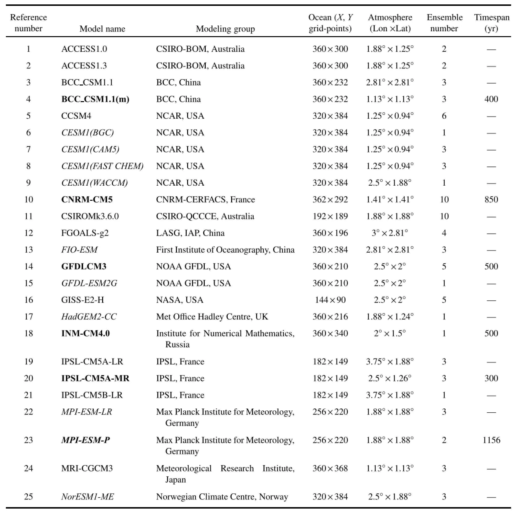
Tab le1.Detailsof the25CMIP5models’“Historical”simulationsand sixmodels’(in bold type)“Pre-industrial”simulationsused in this paper.Themodel names in italic type indicate they are earth system models.

The above-mentioned analyses suggest aw ide range of skillamong themodelsin simulating theobservationalAMO.Modelselection isbased on the follow ing criteria:(1)a significantmultidecadalperiod;(2)a temporalnormalized standard deviationw ithin the rangeof±0.5standard deviationsof the observation;(3)spatial correlationsabove 0.3;(4)spatial normalized standard deviationsw ithin the range of±1 standard deviations of the observation.Table 2 summarizes the selection criteria and shows that six models qualify for selection.These sixmodels[BCC CSM 1.1(m),CNRM-CM 5, GFDLCM 3,INM-CM 4.0,IPSL-CM 5A-MR,andMPI-ESMP]are thereforeemployed to investigate theAMO-related climatic patterns in the internalnaturalsystem.

Fig.1.Power spectrum of the AMO index for the(a)observation(HadISST)and(1–25)themodels.The power spectrum isgiven by theblack line,significantabove the red lineat the5%level.

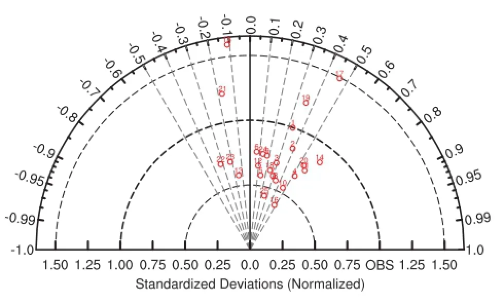
Fig.2.Taylor diagram show ing the temporal features of the AMO index for the period 1874–2001.The x-axis shows the normalized standard deviation and the arc shows the correlation values between observations and the ensemblemean for eachmodel.The red numbers correspond to themodel reference numbers listed in Table 1.

3.2.The AMO in the“Pre-industrial”simulations

Fig.3.Regressions of SST onto the standardized AMO index in the(a)observation and(1–25) models.Black dots indicate statistical significance at the＞95%confidence level,based on the t-test.Theblack frames represent themaximum center in theobservation.Units:°C.

The six models’“Pre-industrial”simulations show one dom inantperiod of20–70 years(Fig.5).Compared to the period of the“Historical”sim ulation foreachmodel,the period of the“Pre-industrial”simulations show s some obvious differences.For example,in the“Historical”simulation,MPI-ESM-P has only one peak period of around 70 years,but in the“Pre-industrial”simulation it hasmultiple significant multidecadal periods.The di ff erencemay be due to the different forcing conditionsbetween the two simulations.Table 3 displays the standard deviationsof the AMO index results. Both in the“Pre-industrial”and“Historical”simulations,the sixmodeled amplitudesareweaker than the observed amplitude(0.15°C).

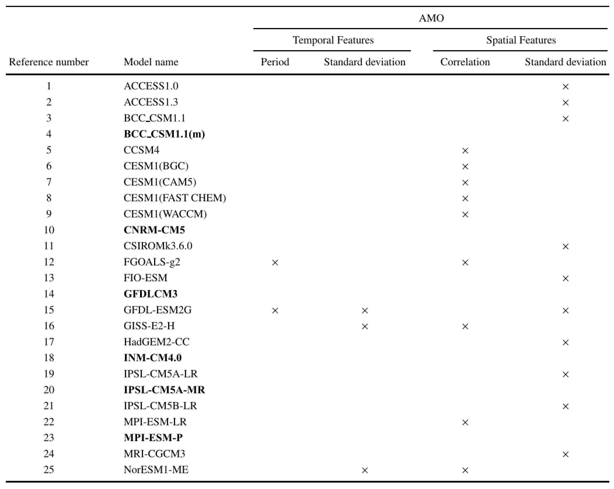
Tab le2.AMO selection criteria for themodels(the six models chosen for the“Pre-industrial”simulations are in bold type).A cross indicates that:(1)themodel has no significantmultidecadal period(third column);(2)the tem poral standard deviation of themodel is outside the range of±0.5 standard deviations of the observation(fourth column);(3)the spatial correlation between the observation and model is less than 0.3(fifth column);and(4)the spatialstandard deviation of themodel isoutside the range of±1 standard deviations of theobservation(sixth column).

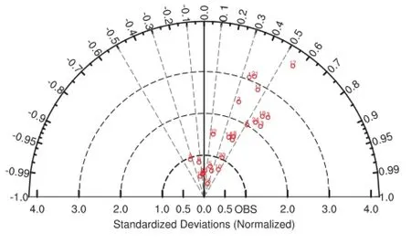
Fig.4.Taylor diagram showing the spatial features of the regressions displayed by Fig.3.Note thatGFDL-ESM 2G has a normalized standard deviation larger than 4.0 and isnotshown.

Table3.Standard deviations of the AMO index in the six selected models’“Historical”and“Pre-industrial”simulations.The standard deviation of the observed AMO index is0.15°C.Units:°C.

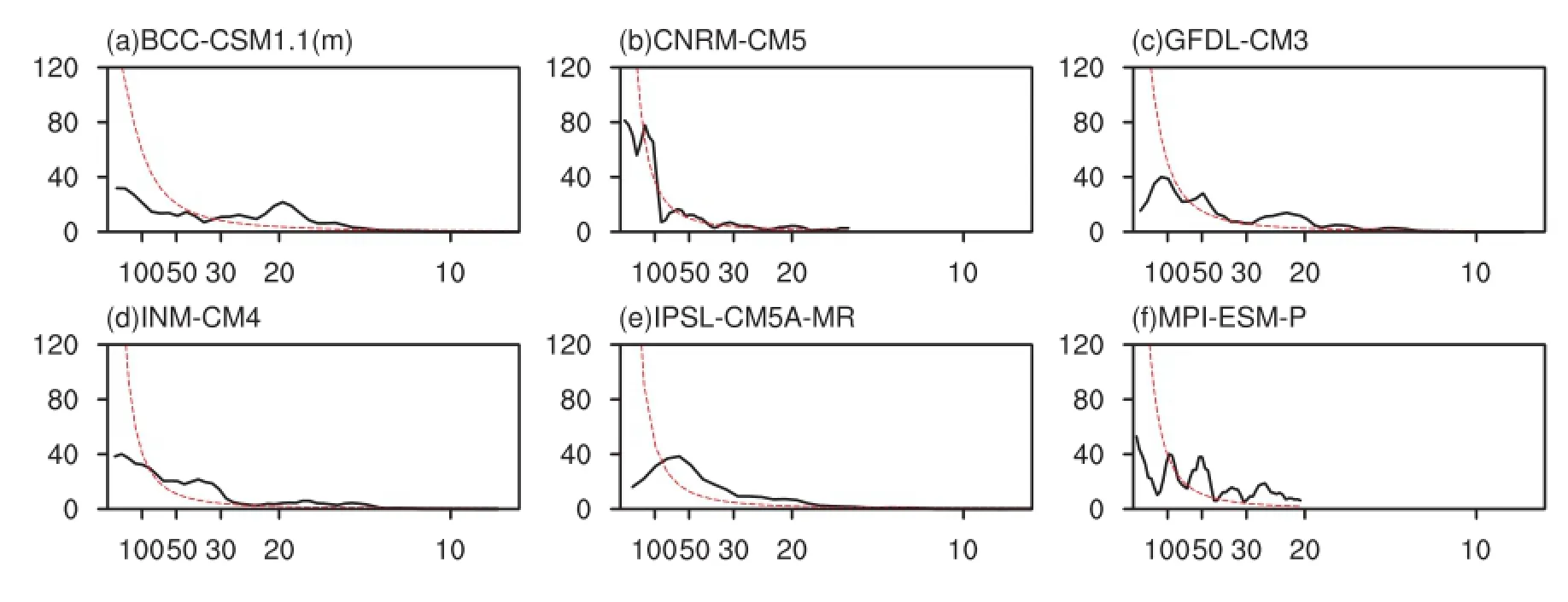
Fig.5.Power spectrum of the AMO index for the six selectedmodels’“Pre-industrial”simulations.The power spectrum isgiven by the black line,significantabove the red line at the 5%level.

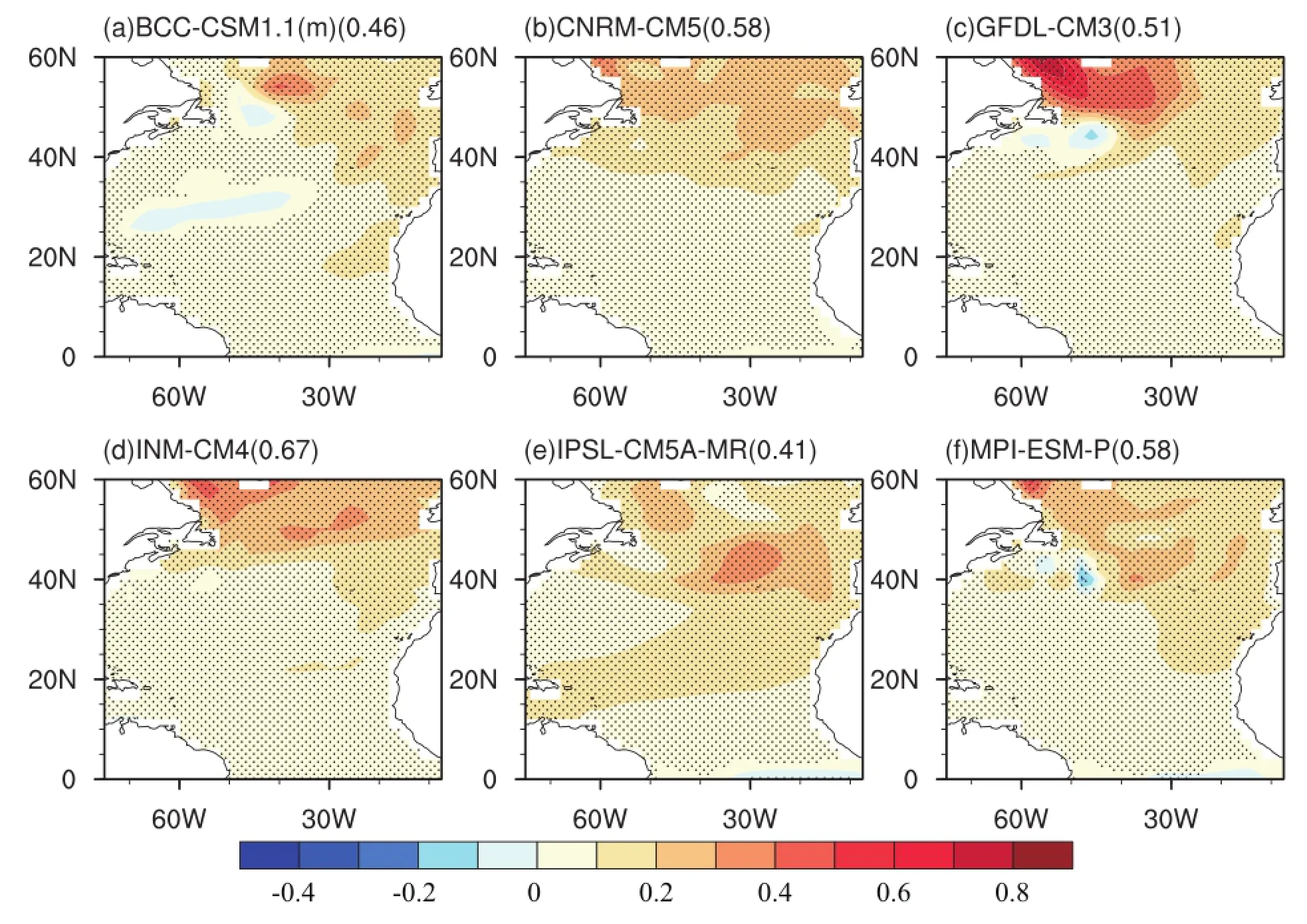
Fig.6.Regressions of SST onto the standardized AMO index in the six selected models’“Pre-industrial”simulations.Black dots indicate statisticalsignificanceat the＞95%confidence level,based on the t-test.Units:°C.

Figure 6 show s the spatial patterns of SST variationsassociated w ith the positive phase of the AMO in the“Preindustrial”simulations.Thedi ff erencesin thespatialpatterns between the“Historical”simulation and observation also exist in the“Pre-industrial”simulation.However,the“Preindustrial”simulations still capture the essential features of theobserved AMO,as indicated by thehigh SCCs from 0.41 to 0.67(Fig.6).It is interesting that the patterns in four of the sixmodels’“Pre-industrial”simulationsare closer to the observation than they are for their“Historical”sim ulations. These analyses indicate the existence of the AMO as an internalmode in the sixmodels,and imply that it is rational to investigate the AMO-related climatic patternsbased on these sixmodels’“Pre-industrial”simulations.

3.3.AMO-related climatic patterns

3.3.1.Surface temperature

Figure7displays theAMO-related spatialpatternsofsurface temperature in the observations in all four seasons.Ondecadal-to-multidecadal timescales,oceanic thermal conditionsplay akey rolein influencing climatevariability(Bjerknes,1964;Gulev etal.,2013).Hence,we first exam ine the AMO-related patterns of surface temperature in the ocean. Theobservationsexhibitanalogousspatialpatternsin allseasons(Fig.7).During positive AMO phases,the SSTs show a basin-scale cooling in the South Atlantic,and amaximum close to theWeddell Sea.For the Pacific,the observations show a tripolar pattern w ith positive temperature anomalies in the North and South Pacific,and slightly negative temper-ature anomalies in the equatorial Pacific(Dong etal.,2006). For the Indian Ocean,thereisawarm signalin bothHadISST (Figs.7a–d)and GISS(Figs.7e–h),though theareaofsignificance ismuch smaller in the former than the latter.

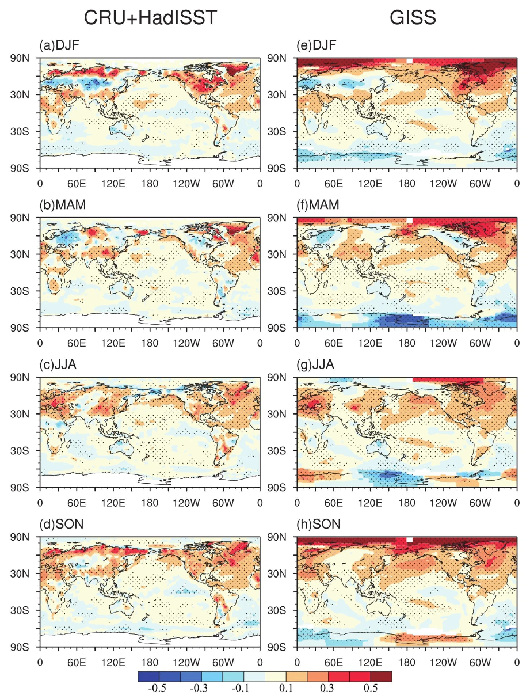
Fig.7.Regressions of surface temperature onto the standardized AMO index:(a–d)CRU(for land temperature)and HadISST(for SST);(e–h)GISS.Black dots indicate statisticalsignificanceat the＞95%confidence level,based on the t-test.Units:°C.

As for the AMO-related surface temperature over land, we focuson theNorthern Hem isphere,considering the larger impacton theNorthern Hem isphere than the SouthernHemisphere and the lower reliability of the data for the Southern Hem isphere compared w ith the Northern Hem isphere for the firsthalf of the 1900s.Observations show increased tem peraturesoverGreenland in all four seasons,maximum anomalies in w inter,andminimum anomalies in summer(Fig.7). Warm ing appearsover thewholeof theNorth American continent inw inter,summerand autumn,while there isan east–westdipolar patternw ith cooling overeastern North America and warming overwestern North America in spring(Fig.7). Warm ing can be found over North Africa in all seasonsexceptsummer(Fig.7).Inw inter,a tripolarpattern isapparent, characterized by warm–cold–warm anomalies from north to south over Eurasia(Figs.7a and e).In spring,the anomalies exhibit an east–west pattern,w ith cooling over Europe and warming overmostof Asia(Figs.7b and f).In summer and autumn,Europe and eastern Asia show positive anomalies, except fora slightcooling over central Asia(Figs.7c–h).In addition,adipolarseesaw of thesurface temperatureover the A rctic and Antarctic isapparentin GISSinw interand spring (Chylek etal.,2010).

To illustrate the regions that have signals that agree among the six models(Figs.S1–S4 in the supporting inform ation),we mark red/blue dots to represent the m atching positive/negative regression coe ffi cients in all of themodels (Fig.8).As can be seen,there is little sim ilarity in the SouthernHem isphereamong themodels,andmatchingpositivesignalsarepresentovermostof theNorthern Hem isphere.The AMO-related SST patterns bear no obvious seasonality and show warm anomaliesover theequatorialPacific,mostof the North Pacific and Indian oceans,in addition to the North Atlantic.For the AMO-related surface temperature over land, it can be seen that there isawarming over Greenland,w ith amaximum extent in w inter and spring and aminimum in summer.Over eastern North America and North A frica,the warm ing exists in all four seasons.For Eurasia,warm ing can be seen in all four seasons over the Scandinavian Peninsula, central Asia and eastern Asia.In particular,there is a band ofwarming from the Scandinavian Peninsula to EastAsia in autumn.

Compared to the observations,a number of di ff erences can be found in themodels.First,themodelsare unable to capture the signalsof the Southern Hemisphere and thenegativesurface temperatureanomalies in theobservations,such as thoseoverwesternNorth America in springandoverEurasia in w inter and spring.Second,there is an opposite signal in the equatorialPacific,in which themodels portray positive anom aliesbut the observationsshow weakly negativeanomalies.However,besides thewarming in the North Atlantic,a number of similarities can be seen between the observations andmodels,such as thewarm ing in theNorth Pacific,Greenland,Scandinavian Peninsula,mostofNorth America,North Africaand EastAsia.

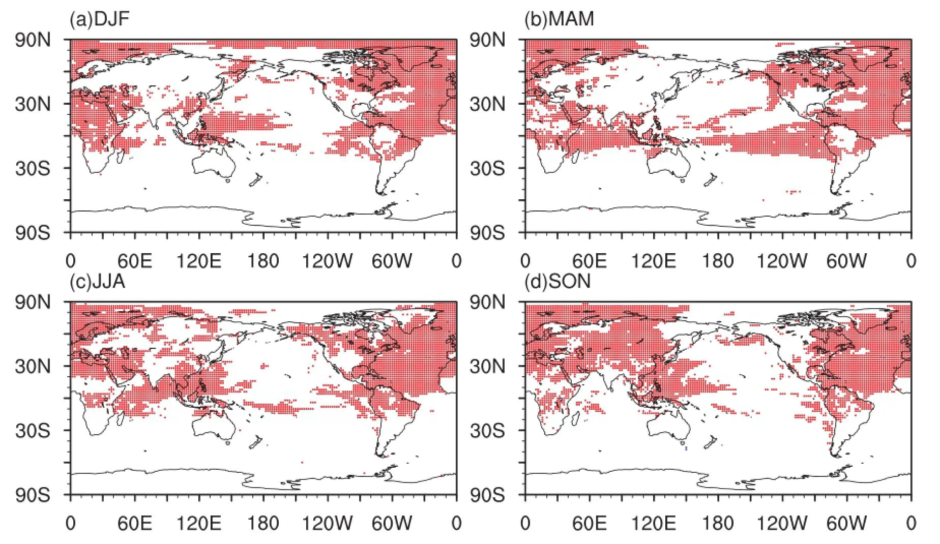
Fig.8.Regression coe ffi cientsof surface tem perature onto the AMO in each of the six selectedmodels,w here the sign of the regression agrees.Red dots indicate positive coe ffi cients.

3.3.2.Precipitation

Given thattheimpactof theAMO onprecipitationmainly occurs in summer and autumn(e.g.,Sutton and Hodson, 2005,2007;Zhang and Delworth,2006;Goswami et al., 2006;Wang et al.,2009;Kavvada et al.,2013),we focus hereondiscussing these two seasons.Figure9shows thespa-tialpattern of precipitationassociated w ith positivephasesof the AMO in the observation.Increased rainfall can be seen over theSaheland northof Brazil,butdecreased rainfallover Brazil,which isa resultof thenorthward shiftof the Atlantic ITCZ(Ting etal.,2011).The amplitude of rainfall over the Sahel is stronger in summer than in autumn.Less rainfall isapparentover North Americain these two seasons.Europe featuresadipolarpattern,w ithm ore rainfalloverwestern Europeand less rainfallovereastern Europe in summer.There is enhanced rainfallover Siberia in summer.For the East Asian summermonsoon,a positive AMO favors intensified rainfall over East Asia,but less rainfall in autumn.In addition,there ismore rainfallover India in the twoseasons,which indicates a latew ithdrawal of the Indian summermonsoon(Lu etal., 2006;Luo etal.,2011).

Similar to Fig.8,Fig.10 displayssignalsof precipitation in the sixmodels(Figs.S5–S6 in the supplementarymaterials)thatagree.Relative to surface temperature,however,the precipitation signalsare less distinct.Enhanced precipitation is situated north of the equator over the A tlantic,im plying a northward shift of the A tlantic ITCZ.M ore rainfall can be seen over theNorth Atlantic,Caribbean Seaand tropicaleastern Pacific,which is related to thewarming in these regions. Moreover,themodelsproduceprecipitation patterns that resemble the observed patternsofmore rainfall over the Sahel and less rainfall over Brazil,and the latew ithdrawal of the Indian summermonsoon.However,more rainfall isapparent over Europe in autumn in themodels,but there is no such significant rainfall in the observation.Additionally,a number of the signals in the observation cannot be found in the models,such as the enhanced rainfall over Siberia in summer.Itshould also bementioned that less rainfallover South China in summer isapparent,which iscontrary to the observational results and previous studies(Lu et al.,2006;Wang etal.,2009;Yu etal.,2009).The reason isunclearand needs to be investigated further.

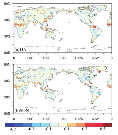
Fig.9.Regressions of precipitation(based on CRU data)onto the standardized AMO index.Black dots indicate statistical significance at the＞95%confidence level,based on the t-test.Units:mm d-1.

4.Summary and discussion

Given thedi ffi cultiesinvolved in removing the impactsof external forcing from the AMO in instrum ental records and historical simulations,the“Historical”and“Pre-industrial Control”simulations of 25 CM IP5 models are used to in-vestigate the AMO as amode ofinternal variability,and its associated climatic impacts.First,we assess the skill of the 25models in simulating the observed AMO,based on their“Historical”simulations.The resultssuggestaw ide rangeof skill among themodels.Sixmodels that demonstrate better skill relative to the othermodelsare selected via certain selection criteria.The“Pre-industrial”simulationsof thesesix m odels also capture the essential features of the AMO,including themultidecadalvariability and basin-scalewarm ing in the North A tlantic.

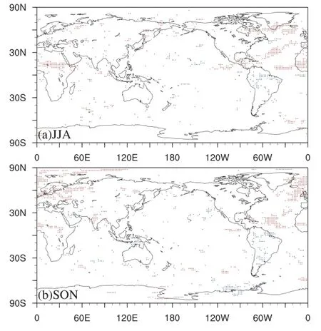
Fig.10.Regression coe ffi cients of precipitation onto the AMO in each of the six selectedmodels,w here the sign of the regression agrees.Red dots indicate positive coefficients,and blue dotsnegative.

The modeled AMO-related surface temperatures show the AMOmay have a larger impacton theNorthern than the Southern Hemisphere.Compared to observations,the distinct di ff erence is the opposite signals in the eastern tropical Pacific,where SSTs play an important role in AMO-related non-local impacts(Zhang and Delworth,2005;Chen et al., 2014).As for thesurface temperatureover land,themain differenceis thatthenegativeanomaliesoverEurasiaand North America in theobservationsare not reproduced in themodels during positive AMO phases.Nonetheless,two key sim ilarities are found:(1)warm ing in the North Pacific;and(2) warming overGreenland,the Scandinavian Peninsula,North A frica,eastern North America,and EastAsia.

Based on the results of the“Pre-industrial”simulations, two hypothesesare proposed.Ding et al.(2014)suggested thatthe recentsurfacewarming inw interovereastern Canada and Greenland is likely caused by the natural climate variability.Here,we also show that thewarming overGreenland isnatural climate variability,but related to the AMO instead of LaNi?na-like SST over the eastern equatorial Pacific.The recent Eurasian cooling has been suggested to be related to the A rctic sea-ice decline(e.g.,Honda et al.,2009;Wu et al.,2013;Gao et al.,2015)and warm ing SSTs in the North Atlantic(Magnusdottiretal.,2004).However,our resultsimply that this recentcoolingmay notbe relatedto thewarm ing SSTs in theNorth Atlantic.

Themodeled AMO-related rainfalldisplaysameridional shiftnorthwardof the Atlantic ITCZ,subsequently leading to more rainfall over the Caribbean Sea and the Sahel,but less rainfall over Brazil.In addition,more rainfall can be found over theNorth Atlantic corresponding to themagnitudeof the warm ing there.This variability of rainfall over land aswell as the increased rainfallover India in autumn in themodels is consistentw ith thatobserved.

In summary,there is good agreement between the observation and models in terms of the AMO-related signalsaround theNorth Atlantic.However,anumberof di ff erences should nevertheless be noted.The reason why the negative surface temperatures related to positive phases of the AMO observed overEurasiaand North Americaarenotreproduced by themodels remains unclear,although three possibilities aresuggested as follows:The first is themodelbias in simulating thebackgroud atmospheric circulation.Kavvada etal. (2013)pointed out thatm odelssuccessfully capturing the observed featuresover the ocean do notnecessarily also capture theobserved atmospheric pattern.Thesecond is the large differencebetween themodelsand observations in termsof the North Pacific SST anomalies,which could influence the surface temperatureoverNorth Americaand Europe through the atmospheric circulation(Frankignouland Senn′echael,2007). And the third is the limitationsof the observationaldata due to short instrumental records,or impacts from external forcing(Suo etal.,2013).

Regarding AMO remote connections,the same signals aremainly shown for the warm ing in the North Pacific and East Asia,aswell as the late w ithdrawalof the Indian summ ermonsoon during positive AMO phases.This is consistenetw ithmany previousstudies(Zhangand Delworth,2005; Lu etal.,2006;Wang etal.,2009;Zhou et al.,2015).The oceanic SST anomaliesmay be the primary cause inducing temperature/rainfall change over East Asia/India(Lu et al., 2006;Lietal.,2008;Zhou etal.,2015).Buthow the AMO links to the SST variationsof theNorth Pacific isunclear.Besides,the impactof the AMO on EastAsiamay beassociated w ith thesurface temperaturechanges from theGreenland Sea to the Kara Sea,linked to sea ice(Lietal.,2015).

The AMO-related surface temperature and precipitation patterns can be found in“Pre-industrial”sim ulations,which means that thesemay be related to internal climate variability.The AMO isconsidered asa vitaldecadal-scalepredictor because of its low-frequency nature(Keenlysideetal.,2008; Hurrelletal.,2009;Meehletal.,2009;Kavvadaetal.,2013). This study provides clues for decadal prediction in regions mainly influenced by internalclimatevariability,on thebasis of the view that the real climate consists of natural internal variability and external forcing(Luo and Li,2014;Steinman etal.,2015).

Acknow ledgements.Weacknow ledge the two anonymous reviewersand Prof.Noel KEENLYSIDE for providing valuable comments on an earliermanuscript.This study was jointly supported by the National Natural Science Foundation of China(Grant No. 41421004),the National Key Basic Research Development Program of China(GrantNo.2016YFA0601802 and 2015CB453202), and the National Natural Science Foundation of China(Grant Nos. 41375085).

E lectronic supplementarymaterial.Supplementarymaterial is available in the online version of this article at:http://dx.doi.org/ 10.1007/s00376-016-5270-4.

A llen,R.J.,2015:A 21st century northward tropical precipitation shift caused by future anthropogenic aerosol reductions.J. Geophys.Res.Atmos.,120,9087–9102,doi:10.1002/2015JD 023623.

Ba,J.,and Coauthors,2014:A multi-model comparison of Atlanticmultidecadalvariability.Climate Dyn.,43,2333–2348, doi:10.1007/s00382-014-2056-1.

Bjerknes,J.,1964:Atlantic air-sea interaction.Advances in Geophysics,10,1–82.

Booth,B.B.B.,N.J.Dunstone,P.R.Halloran,T.Andrew s,and N.Bellouin,2012:Aerosols im plicated as a prime driver of twentieth-century North Atlantic climate variability.Nature, 484,228–232.

Chen,W.,R.Y.Lu,and B.W.Dong,2014:Intensified anticyclonic anomaly over the western North Pacific during El Ni?no decaying summer under a weakened A tlantic thermohaline circulation.J.Geophys.Res.Atmos.,119,13 637–13 650,doi: 10.1002/2014JD022199.

Cheng,W.,J.C.H.Chiang,and D.X.Zhang,2013:Atlantic meridional overturning circulation(AMOC)in CMIP5models:RCP and historical simulations.J.Climate,26,7187–7197.

Chiang,J.-C.-H.,C.-Y.Chang,and M.-F.Wehner,2013:Longterm behavior of the Atlantic interhem ispheric SST gradient in the CMIP5 historical simulations.J.Climate,26,8628–8640.

Chylek,P.,C.K.Folland,G.Lesins,and M.K.Dubey,2010: Twentieth century bipolar seesaw of the A rctic and Antarctic surface air temperatures.Geophys.Res.Lett.,37,L08703, doi:10.1029/2010GL042793.

Chylek,P.,C.K.Folland,H.A.Dijkstra,G.Lesins,and M.K. Dubey,2011:Ice-core dataevidence fora prom inentnear20 year time-scaleof the AtlanticMultidecadalOscillation.Geophys.Res.Lett.,38,L13704,doi:10.1029/2011GL047501.

Delworth,T.L.,and M.E.Mann,2000:Observed and simulated multidecadalvariability in the Northern Hem isphere.Climate Dyn.,16,661–676.

Ding,Q.H.,J.M.Wallace,D.S.Battisti,E.J.Steig,A.J.E. Gallant,H.J.Kim,and L.Geng,2014:Tropical forcing of the recent rapid Arctic warm ing in northeastern Canada and Greenland.Nature,509(7499),209–212.

Dong,B.W.,R.T.Sutton,and A.A.Scaife,2006:Multidecadal modulation of ElNi?no-SouthernOscillation(ENSO)variance by Atlantic Ocean sea surface temperatures.Geophys.Res. Lett.,33,L08705,doi:10.1029/2006GL025766.

Drinkwater,K.F.,M.M iles,I.M edhaug,O.H.Otter?,T.Kristiansen,S.Sundbya,and Y.Q.Gao,2014:TheAtlanticMultidecadal Oscillation:Itsmanifestations and impactswith special emphasis on the Atlantic region north of 60°N.Journal ofMarine Systems,133,117–130.

Dunstone,N.J.,D.M.Smith,B.B.B.Booth,L.Hermanson, and R.Eade,2013:Anthropogenic aerosol forcing of Atlantic tropicalstorms.Nature Geoscience,6(7),534–539.

Enfield,D.B.,A.M.Mestas-Nu?nez,and P.J.Trimble,2001:The Atlantic Multidecadal Oscillation and its relation to rainfall and river flows in the continental U.S.Geophys.Res.Lett., 28(10),2077–2080.

Feng,S.,and Q.Hu,2008:How the North Atlantic M ultidecadal Oscillation may have influenced the Indian summer monsoon during the past twom illennia.Geophys.Res.Lett.,35, L01707,doi:10.1029/2007GL032484.

Frankignoul,C.,and N.Senn′echael,2007:Observed influence of North Pacific SST anomalies on the atmospheric circulation. J.Climate,20,592–606,doi:10.1175/JCLI4021.1.

Gao,Y.Q.,and Coauthors,2015:Arctic sea ice and Eurasian climate:A review.Adv.Atmos.Sci.,32(1),92–114,doi: 10.1007/s00376-014-0009-6.

Goswam i,B.N.,M.S.Madhusoodanan,C.P.Neema,and D. Sengupta,2006:A physicalmechanism for North Atlantic SST influenceon the Indian summermonsoon.Geophys.Res. Lett.,33,L02706,doi:10.1029/2005GL024803.

Gray,S.T.,L.J.Graum lich,J.L.Betancourt,and G.T.Pederson, 2004:A tree-ring based reconstruction of the Atlantic Multidecadal Oscillation since 1567 A.D.Geophys.Res.Lett.,31, L12205,doi:10.1029/2004GL019932.

Gulev,S.K.,M.Latif,N.Keenlyside,W.Park,and K.P.Koltermann,2013:North Atlantic Ocean control on surface heat flux onmultidecadal timescales.Nature,499(7459),464–467.

Hansen,J.,M.Sato,R.Ruedy,K.Lo,D.Lea,and M. Medina-Elizade,2006:Global temperature change.Proceedings of the National Academy of Sciences of the United States ofAmerica,103,14 288–14 293,doi:10.1073/pnas. 0606291103.

Honda,M.,J.Inoue,and S.Yamane,2009:Influenceof low Arctic sea-icem inima on anomalously cold Eurasian w inters.Geophys.Res.Lett.,36,L08707,doi:10.1029/2008GL037079.

Hurrell,J.W.,and Coauthors,2009:Decadal climate prediction: Opportunitiesand challenges.Proc.OceanObs’09:Sustained OceanObservationsand Information for Society,ESA Publication,Venice,521–533.

Kavvada,A.,A.Ruiz-Barradas,and S.Nigam,2013:AMO’s structureand climate footprintin observationsand IPCCAR5 climate simulations.Climate Dyn.,41(5–6),1345–1364.

Keenlyside,N.S.,M.Latif,J.Jungclaus,L.Kornblueh,and E. Roeckner,2008:Advancing decadal-scale climate prediction in the North A tlantic sector.Nature,453:84–88.

Knight,J.R.,C.K.Folland,and A.A.Scaife,2006:Climate impactsof the Atlantic MultidecadalOscillation.Geophys.Res. Lett.,33,L17706,doi:10.1029/2006GL026242.

Li,F.,H.J.Wang,and Y.Q.Gao,2015:Extratropicaloceanwarming and winter Arctic sea ice cover since the 1990s.J.Climate,28,5510–5522,doi:10.1175/JCLI-D-14-00629.1.

Li,S.L.,and G.T.Bates,2007:Influence of the Atlanticmultidecadal oscillation on thew inter climate of EastChina.Adv. Atmos.Sci.,24(1),126–135,doi:10.1007/s00376-007-0126-6.

Li,S.L.,J.Perlwitz,X.W.Quan,and M.P.Hoerling,2008:Modelling the influence of North A tlanticmultidecadalwarm th on the Indian summer rainfall.Geophys.Res.Lett.,35,L05804, doi:10.1029/2007GL032901.

Lu,R.Y.,B.W.Dong,and H.Ding,2006:Impact of the Atlantic Multidecadal Oscillation on the Asian summermonsoon.Geophys.Res.Lett.,33,L24701,doi:10.1029/2006GL 027655.

Luo,F.F.,and S.L.Li,2014:Joint statistical-dynam ical approach to decadal prediction of East Asian surface air temperature.Science China Earth Sciences,57,3062–3072,doi: 10.1007/s11430-014-4984-3.

Luo,F.F.,S.L.Li,and T.Furevik,2011:The connection between the A tlantic M ultidecadalOscillation and the Indian summer monsoon in Bergen ClimateModel Version 2.0.J.Geophys. Res.,116,D19117,doi:10.1029/2011JD015848.

Magnusdottir,G.,C.Deser,and R.Saravanan,2004:The e ff ects of North Atlantic SST and sea ice anomalies on the winter circulation in CCM 3.Part I:Main features and storm track characteristicsof the response.J.Climate,17,857–876.

Martin,E.R.,C.Thorncroft,and B.B.B.Booth,2014:TheMultidecadal A tlantic SST–Sahel rainfall teleconnection in CM IP5 simulations.J.Climate,27,784–806.

Medhaug,I.,and T.Furevik,2011:North Atlantic 20th century multidecadal variability in coupled climatemodels:Sea surface temperature and ocean overturning circulation.Ocean Science Discussions,8,353–396.

M eehl,G.A.,and Coauthors,2009:Decadal prediction:Can itbe skillful?Bull.Amer.Meteor.Soc.,90,1467–1485.

M itchell,T.D.,and P.D.Jones,2005:An improved method of constructing a database ofmonthly climateobservations and associated high-resolution grids.International JournalofClimatology,25,693–712,doi:10.1002/joc.1181.

M sadek,R.,C.Frankignoul,and L.Z.X.Li,2011:Mechanism sof theatmospheric response to North Atlanticmultidecadalvariability:A model study.Climate Dyn.,36,1255–1276,doi: 10.1007/s00382-010-0958-0.

Otter?,O.H.,M.Bentsen,H.Drange,and L.L.Suo,2010:External forcing asametronome for Atlanticmultidecadalvariability.Nature Geoscience,3,688–694.

Rayner,N.A.,D.E.Parker,E.B.Horton,C.K.Folland,L. V.A lexander,D.P.Rowell,E.C.Kent,and A.Kaplan, 2003:Global analyses of sea surface temperature,sea ice, and nightmarineair temperaturesince the latenineteenth century.J.Geophys.Res.,108(D14),4407,doi:10.1029/2002JD 002670.

Steinman,B.A.,M.E.M ann,and S.K.M iller,2015:A tlantic and Pacific multidecadal oscillations and Northern Hemisphere temperatures.Science,347(6225),988–991.

Suo,L.L.,O.H.Otter?,M.Bentsen,Y.Q.Gao,and O.M.Johannessen,2013:External forcing of the early 20th century arctic warm ing.Tellus A,65,20578.

Sutton,R.T.,and D.L.R.Hodson,2005:Atlantic Ocean forcing of North American and European summer climate.Science, 309,115–118.

Sutton,R.T.,and D.L.R.Hodson,2007:Climate response to basin-scalewarm ing and coolingof theNorth AtlanticOcean. J.Climate,20,891–907.

Taylor,K.E.,2001:Summarizingmultipleaspects ofmodel performance in a single diagram.J.Geophys.Res,106,7183–7192.

Taylor,K.E.,R.J.Stou ff er,G.A.Meehl,2012:An overview of CM IP5 and the experiment design.Bull.Amer.Meteor.Soc., 93,485–498.

Ting,M.F.,Y.Kushnir,R.Seager,and C.H.Li,2009:Forced and internal twentieth-century SST trends in theNorth Atlantic.J. Climate,22,1469–1481.

Ting,M.F.,Y.Kushnir,R.Seager,and C.H.Li,2011:Robust featuresof Atlanticmulti-decadal variability and its climate impacts.Geophys.Res.Lett.,38,L17705,doi:10.1029/2011GL 048712.

Wang,Y.M.,S.L.Li,and D.H.Luo,2009:Seasonal response of Asianmonsoonal climate to the Atlantic MultidecadalOscillation.J.Geophys.Res.,114,D02112,doi:10.1029/2008JD 010929.

Wilcox,L.J.,E.J.Highwood,and N.J.Dunstone,2013:The influence of anthropogenic aerosolonmulti-decadal variations of historicalglobal climate.Environmental Research Letters, 8(2),024033.

Wu,B.Y.,R.H.Zhang,R.D’Arrigo,and J.Z.Su,2013:On the Relationship betweenwinter sea iceand summeratmospheric circulation over Eurasia.J.Climate,26,5523–5536.

Yu,L.,Y.Q.Gao,H.J.Wang,D.Guo,and S.L.Li,2009:The responsesof East Asian Summermonsoon to the North A tlantic M eridional Overturning Circulation in an enhanced freshwater input simulation.Chinese Science Bulletin,54,4724–4732,doi:10.1007/s11434-009-0720-3.

Zhang,L.P.,and C.Z.Wang,2013:Multidecadal North Atlantic sea surface temperature and Atlantic meridional overturning circulation variability in CM IP5 historical simulations.J. Geophys.Res.Oceans,118,5772–5791,doi:10.1002/jgrc. 20390.

Zhang,R.,and T.L.Delworth,2005:Simulated tropical response to asubstantialweakening of theAtlantic thermohaline circulation.J.Climate,18,1853–1860.

Zhang,R.,and T.L.Delworth,2006:Impact of A tlantic multidecadaloscillationson India/Sahel rainfalland Atlantic hurricanes.Geophys.Res.Lett.,33,L17712,doi:10.1029/2006GL 026267.

Zhou,X.M.,S.L.Li,F.F.Luo,Y.Q.Gao,and T.Furevik,2015: Air-sea coupling enhances the East Asian w inter climate response to the Atlantic Multidecadal Oscillation.Adv.Atmos. Sci.,32(12),1647–1659,doi:10.1007/s00376-015-5030-x.

:Han,Z.,F.F.Luo,S.L.Li,Y.Q.Gao,T.Furevik,and L.Svendsen,2016:Simulation by CMIP5models of the Atlantic Multidecadal Oscillation and its climate impacts.Adv.Atmos.Sci.,33(12),1329–1342,

10.1007/s00376-016-5270-4.

(Received 15December2015;revised 18 June2016;accepted 8 July 2016)

?Corresponding author:Feifei LUO

Email:luofeifei212@mail.iap.ac.cn

?Institute ofAtmospheric Physics/Chinese Academy of Sciences,and Science Press and Springer-Verlag Berlin Heidelberg 2016