Paromita Chakraborty, Arindam Sarkar

1. School of Civil Engineering, Kalinga Institute of Industrial Technology (KIIT) Deemed to be University,Bhubaneswar, Odisha, India

2. School of Infrastructure, Indian Institute of Technology (IIT) Bhubaneswar Aurgul, Bhubaneswar, Odisha, India

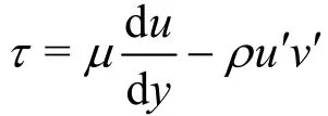
Abstract: Flow through submerged rigid vegetation has been studied both analytically and experimentally. The Reynolds stress,present in the governing equation, has been modeled using one of the turbulent stress equations, adopted in numerous cases. The advantage of this turbulent stress model is to replace the mixing length nonlinear term of the stress with a linear relation between stress and the velocity gradient. The velocity field and shear stress are obtained by solving the governing force balance equation numerically.A correlation, validated with the experimental results, has been developed for the relevant non-dimensional numbers.

Key words: Submerged vegetation, Reynolds stress, drag force, stream wise velocity

Introduction

Flow through aquatic vegetation has been an area of active research due to its wide spread application in the fields of flood control, resistance to soil erosion,water pollutant control and many others. In the study of this phenomenon, it is essential to estimate the drag coefficient and the turbulent stress. To estimate the turbulent stress, mainly the mixing length theory is employed, but the mixing length in the vegetated flow differs for different flow situations and this has attracted several researchers over the years. Huai et al.[1]investigated flow through submerged rigid vegetation considering a four zone model. Mixing length scales for different zones have been estimated and velocity field has been obtained for different cases numerically. Hu et al.[2]constructed a three layer model and proposed an approximate analytical solution using power series method for the upper vegetation layer. An exact solution for the nonvegetated layer has also been put forward for the velocity and the shear stress. Hsieh and Shiu[3]introduced a new idea by implementing Biot’s theory of poro elasticity to formulate the governing equations of flow field within the vegetated area. By this method,the drag force is inherently introduced into the equation by the porosity factor. Heish et al.[3]considered both laminar and turbulent flow and the turbulent stress was modeled by a linear relation of stress and velocity gradient. The governing equation was solved analytically and the effect of various parameters on the velocity had been analyzed. Hsieh[4]also carried out an investigation on turbulent emergent and non-emergent vegetated flow using the Biot’s theory. Effect of vegetation on the flow field was analyzed and reported that the turbulent strength increases with increase of the Reynolds stresses,which results in uniform distribution of the streamwise velocity profiles. Rowinski and Kubrak[5]developed a 1-D model using a modified mixing length theory for predicting the vertical velocity distribution for flow through emergent vegetation.Nazu and Nakagawa[6]put forward a three dimensional model combining mass, momentum and energy conservation equations. Other 3-D turbulence models including k-ε model[7-8]and large eddy simulation (LES)[9-11]etc. were also introduced for the study of flow field of both submerged and emerged vegetation. Though these 3-D models can yield relatively more accurate results, the level of complexity is more. Simple 1-D models are relatively easier to solve and can produce results with reasonable accuracy.

Researchers have also examined various effects like the formation of shear layer, vortex structure to understand their effect on the velocity, bed shear, etc..Ghisalberti and Nepf[12]discussed the effect of vortex structure, which was formed due to the growth of the shear layer, on the flexible vegetated layer. Bouma et al.[13]performed experiment in laboratory flume and also did field experiments on the vegetation patches which were replicated with a modified k-ε model.The model was able to study the flow field except those at the leading edge of the vegetation. Souliotis and Prinos[14]used Fluent to investigate the effect of a vegetation patch density and the length of the patch on the development of flow and turbulence characteristics. Recently, Guo and Zhang[15]first solved Navier-Stokes equation for laminar flow and then modified that to include the effect of turbulence.Nepf[16]rigorously analyzed the effect of hydrodynamics of the various flow conditions on individual plant and vegetation patches and found that flow resistance is more in the patch-scale vegetation distribution, than the geometry considered in the individual plants. Nepf and Vivoni[17]also considered the flow structure in depth limited flow and proposed an empirical formula for the determination of the constant velocity height for the lower vegetated zone.

In the present study, the flow through submerged rigid vegetation has been investigated both experimentally and numerically. acoustic Doppler velocimeter(ADV) was used to measure the velocity field within the vegetation array. For numerical investigation, the governing differential equation is formed by balancing the forces acting on the fluid element which are mainly gravity force, drag force and the force due to the Reynolds stress. For solving the force balance equation, a linear turbulent stress model has been introduced. The velocity and shear stress have been obtained from the numerical solutions of the formulated equations. The pertinent dimensionless parameters governing the flow phenomena have been identified and a correlation has been established using the available experimental data in the literature. The correlation has been validated by comparing the predicted velocity fields with those of the experimental investigation. The shear stress distributions for the corresponding cases have also been obtained.

1. Experimentation

The flume, utilized for carrying out the experiments, is a tilting open channel rectangular flume of 10 m length, 0.4 m wide, and 0.8 m height. A digital flow meter, connected to the electrical input of the pump, has been employed to maintain a constant flow rate though the flume. Water is circulated through the flume at a constant flow rate maintained by a digital flow meter which is connected to the electrical input of the pump. For convenience in measurement, the walls of the flume are made of glass. The model of random rigid vegetation array is located at a distance of 1.3 m from the entrance of the flume. PVC cylinders of 6 mm diameter and 18 mm height are used to model the submerged rigid vegetation, these cylinders are fixed on a horizontal plexiglass plate of 20 mm thickness rendering the effective height of the cylinders as 16 mm. The plexiglass plate is placed in the bottom of the flume. For all the experimental runs,the cylinders are completely submerged in the flow.The depth of water is 0.32 m. For measuring the free surface flow, a point gauge of accuracy ±0.1 mm is used. For different discharge and cylinder diameters,experiments have been carried out. The results of the two runs are reported in the present study. The glass cylinders are distributed throughout the entire width of the plate. The cylinders are placed randomly and the locations of the cylinders are fixed from random numbers, generated by a MATLAB code. The minimum center line distance between the cylinders and the distance between the wall and the centre of the cylinder are fixed accordingly as taken in the investigation of Sarkar[18]. The number density of the cylinder arrays is taken as 0.09 cylinders/m2for all the experiments, which lies in the range of 200 plants/m2-2 000 plants/m2[19]. Downlooking Micro ADV of 16 MHz is employed for the measurement of the streamwise point velocity component. For measuring at any vertical and longitudinal section along the flume, the ADV is placed on a traverse mechanism for convenience in adjustment if any. The time independent average velocity is measured at each location keeping sampling durations at various locations in between 3 min -6 min, this duration depends on the localized turbulence intensity. The undisturbed velocity distribution at a section far upstream of the submerged cylinder are also measured and compared with the logarithmic law, which may be written as follows

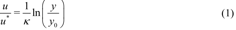
where u is the streamwise velocity component along x,*

u is the shear velocity, κ is the von Karman constant (=0.41), y0is the zero velocity level from the bed along y. Following van Rijn[20], y0is written as

where ν is kinematic viscosity.

The streamwise velocity data within the wall shear layer (=0.2) are used to determine the shear velocity, whereis y/ h. The curve fitted to the measured data within the wall shear layer is as follows

where C is a constant,*u is calculated as 0.016 m/s.

Figure 1 compares the distribution of the measured longitudinal velocity component with logarithmic law, which agrees well with the logarithmic law.The observed downward shift is due to the roughness of the bed as was also pointed out by Ashtiani et al.[21].

Fig. 1 Logarithmic profile validation

Figure 1 compares the distribution of the measured longitudinal velocity component with logarithmic law, which agrees well with the logarithmic law. The observed downward shift is due to the roughness of the bed as was also pointed out by Ashtiani et al.[21].

2. Velocity distribution

Velocity measurements have been carried out using ADV at various locations across the array as well as before entering the array as shown in Fig. 2(b).Out of several runs, run 1, run 2 is being reported here.These two runs are considered here, due to the wide range of flow conditions. In both cases, depth of flow is considered to be constant, by adjusting the height of the tail gate as mentioned in Table 1. The streamwise velocity component (u) measurements are taken along vertical sections within the randomly distributed submerged cylinders as shown in Fig. 2(a), where x,y are the longitudinal and vertical directions. The non-dimensional vertical distributions of streamwise velocity component are plotted.

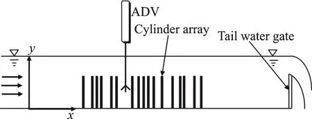
Fig. 2(a) Schematic diagram of the experimental setup showing the elevation

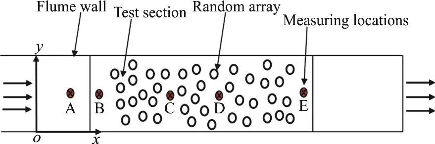
Fig. 2(b) (Color online) Schematic of the experimental setup showing the plan and measuring locations

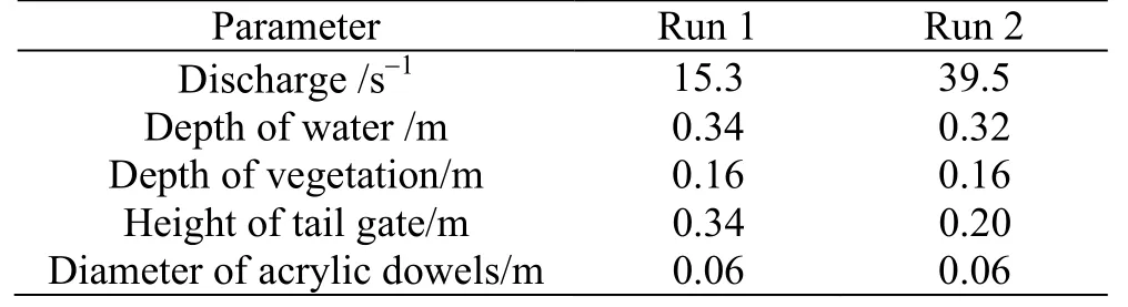
Table 1 Calculation parameters for different runs for submerged rigid randomly distributed vegetation with rigid vegetation

Figure 3 depicts the stream wise velocity distribution for a particular run at different sections across the array. It is found that in both the runs 1, 2, the velocities outside the array i.e., the sections A, B,represent the open channel velocity distributions, but the velocity within the array i.e., sections C, D is relatively less due to the resistance offered by the vegetated layer.

Figure 4(a) presents the non-dimensional streamwise velocity distributions for the location C within the array for run1, run 2 of the present experiment.Whereas, Fig. 4(b) represents the non-dimensional streamwise velocity distribution for various runs of present study and the comparisons of the velocity profiles with the previous studies with submerged and emerged regular square shape distribution of rigid vegetation. From both Figs. 4(a), 4(b), it is observed that the flow resistance for the randomly distributed submerged vegetation is more compared with to the regular pattern distribution of submerged vegetation within the vegetation array. From both Figs. 4(a), 4(b),it is observed that the flow resistance for the present study is more due to the higher vegetation density(265 m2) compared with the study of Huai et al.[3](200 m2), while other parameters remaining the same in both experiments. For the emergent vegetation, it is found that the streamwise velocity component within the vegetation is even more compared with the randomly distributed submerged vegetation as shown in Fig. 4(b). Figure 4(c) shows the comparison of present experiments with the previous studies and it is observed that the non-dimensional experimental velocities follow the same trend.

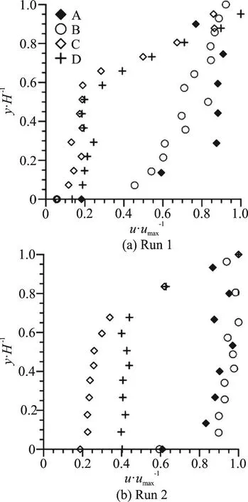
Fig. 3 Non-dimensional streamwise velocity profiles at various locations

3. Problem formulation

Figure 5 depicts the schematic of the model used for the problem formulation. The domain has been divided in three layers which are lower vegetation,upper vegetation and non-vegetated zone respectively.The flow is assumed to be turbulent, incompressible,and fully developed. The reference frame has been chosen as shown in the Fig. 1. H is the total depth of water, h1is the height of the non-vegetated layer,h2and hcare the heights of upper and lower vegetated layer respectively.

3.1 Governing equations

The lower vegetation layer is very near to the solid bed surface and the effect of the turbulence is small compared with the gravity and drag forces acting on the fluid element. Therefore, neglecting the body force, the force balance equation on the fluid in this layer is simply written as

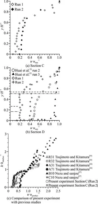
Fig. 4 Non-dimensional streamwise velocity profiles for different runs (a) Section C, (b) Section D and (c) Comparison of present experiments with previous studies

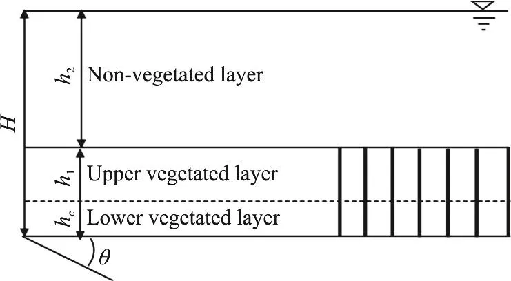
Fig. 5 Schematic diagram of submerged rigid vegetation over plane bed

where F, ρ, g and s are drag force per unit volume, density of water, acceleration due to gravity and bed slope respectively.

Vegetation drag force in the upper vegetation layer has been estimated as

where CDis the drag coefficient, a is the vertically averaged projected vegetation area per unit volume and u is the average velocity in the stream wise direction.

3.1.1 Lower vegetated layer

In this layer, velocity is assumed to be constant and it is obtained from Eq. (4) and Eq. (5) as

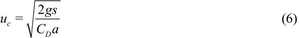
The height of lower vegetated layer, which is considered as weak turbulence zone has been estimated from Nepf[16]experimental study of rigid submerged vegetation as

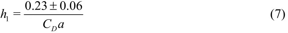
Several studies have been conducted to determine the constant height of lower vegetation. Huai et al.[1]modified the Eq. (7) for regular square pattern array of vegetation as

where p is the relative spacing between the two adjacent plants.

In the present study, Eq. (8) is further modified for the random distribution of vegetation as

where dvis the characteristic length of the randomly distributed vegetation, which is being calculated following Serra et al.[22]and Sarkar[18]approximate formula for random array.

3.1.2 Upper vegetated layer

Adjacent to the vegetation-water interface, a shear layer formation takes place due to the vegetation drag causing vortex structure. The vortex penetration depth along the vegetation layer is termed as the upper vegetation layer. In this layer drag force is dominant and balances the gravity and shear stress. Therefore,the equation governing the flow phenomena in this layer can be obtained as follows

where1τ denotes the shear stress, u1denotes the velocity in the upper vegetation layer.

3.1.3 Non-vegetated layer

In this layer vegetation drag is absent and the shear stress is balanced by gravity. Therefore the governing equation is as follows

where2τ denotes the shear stress in the nonvegetated layer. This shear stress is the combination of the laminar as well as turbulent shear stress. Various theories[23-25]have been proposed by the researchers to model the turbulent shear stress. Heish[4]used a turbulence model, which linearizes the turbulent stress resulting in less computational or analytical effort for solving the equation. Substituting shear stress as

in Eq. (10), Eq. (11) and using the turbulent stress theory used by Heish[3-4]

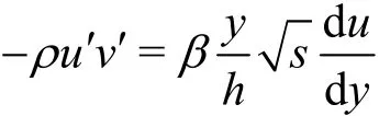
we get the equations as follows:

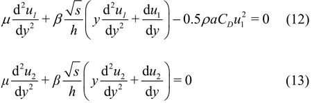
3.1.4 Boundary conditions

Equations (12), (13) are 2ndorder, non-linear ODEs, each of which requires two boundary conditions to get the solution. In the lower vegetation layer the velocity is constant. At the starting point of the upper vegetation layer the velocity of water will be the same as the constant velocity of the lower vegetation water. The relevant boundary conditions to solve the equations are given as follows

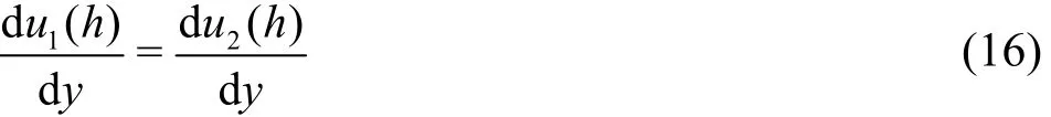
Applying continuity of the velocity at the interface of the vegetated and non-vegetated layer

Deriving from the continuity of the stress, the shear stress equation is obtained as

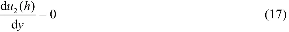
At the free surface, velocity gradient is nearly zero

3.2 Solution

For solving Eqs. (12), (13), the followings are substituted:

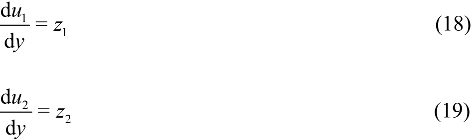
and the following system of equations are obtained:

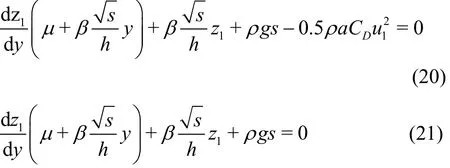
Rearranging the terms we get the equations as follows:

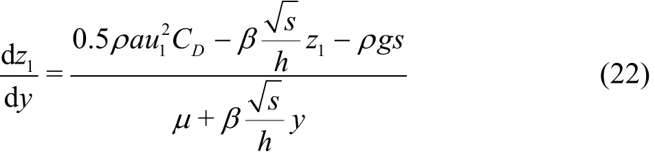
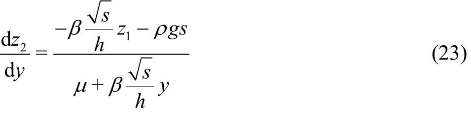
The two 2ndorder ODEs have been converted to four 1storder ODEs (Eqs. (18), (19), (22) and (23)).This set of equations is solved numerically. First, the equations are discretized as follows:

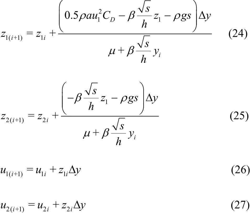
where i denotes the grid point at y. Δy denotes the difference between the two consecutive grid points.The equations are discretized following the Euler’s scheme. The accuracy has been ensured by selecting optimum grid size after grid independence test.

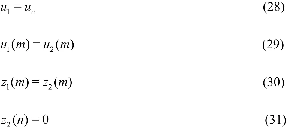
where m, n denote the grid points of the interface and the free surface respectively.

The system of equations subjected to the boundary conditions are solved by shooting method. The grid size in the y direction is chosen by taking 500 points. Grid independence test is carried out by changing the grid size. When the difference between the velocities of different runs is less than 10-5, the optimum grid is selected.

Table 2 Calculation parameters for different experiments with rigid vegetation [7, 26-27]

4. Calibration

In the equation of the turbulent stress, β is unknown. Heish[4]calibrated the value of β for emerged vegetation considering the experimental results of the previously reported investigations.However, a single value of β has been given for a set of parameters. The range of parameters was relatively small as a single value of β cannot predict wide range of data with reasonable accuracy. In the present study, a correlation has been developed so that β can be estimated for a wider range of data with reasonable accuracy. In this section, first calibration has been carried out for β considering data from previous studies[7,26-27]. Table 2 presents different values of β for the corresponding flow situations.The relevant dimensionless numbers have been defined and using the experimental results, a correlation has been established for estimating the value of β.

Figure 6 depicts the calibrations for β for different cases considered. It is evident from the graph, that the calculated values of the steam wise velocities are well matched with the experimental results for the tabulated values of β for different cases.

5. Dimensionless numbers

To form the dimensionless numbers, the governing equations are made dimensionless. In this regard,the following variables are made non-dimensional

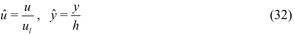
The pertinent non-dimensional numbers governing the flow are obtained as follows:

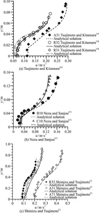
Fig.6 Calibrations of β for different cases

Table 3 Parameters considered for the validation of the model

Using the data listed in Table 1, the following co-relation has been obtained with a correlation coefficient2=0.85

R

6. Validation

The correlation proposed is validated for few experimental runs. For validation purpose, the experiment (A71) of Tsujimoto and Kitamura[26]and the experimental results of the present study have been considered. Using the data of Tsujimoto and Kitamura[26]N1is 889.5002, N2is 34 371.71 and N3=139588.4. From this β is estimated to be 9.45.Parameters involved for the calculation of β are shown in the Table 3. Using β =9.45, the stream wise velocity distribution is plotted with the experimental results of Tsujimoto and Kitamura[26]as shown in the Fig. 7(a). For Run1 of the present experimental study, to estimate the characteristic length of the randomly distributed vegetation, the method followed in the work of Sera et al.[22]has been implemented and the relevant parameters are obtained as follows, solid plant fraction SPF=0.02545, characteristic length of the randomly distributed vegetation is found to be 0.06146 m and vertically averaged projected vegetation area per unit volume a=1.52 m-1. These parameters are utilized to determine the depth of lower vegetated layer using Eq. (9) as discussed in section(governing equations). It is well-known that the velocity remains nearly constant upto a certain height from the bed. The magnitude of the height varies for different flow situations, which affects the velocity field of the upper vegetation significantly. Due to this,numerous researchers carried out extensive investigation on this. Out of the several investigations, the empirical formula of Nepf[16]has been widely used,which is already mentioned in Eq. (7).

Using Eq. (9) in the present study lower vegetation height has been estimated to be 0.11 m which matches very well with the experimental result as shown in the Fig. 7(a). This also justifies the suitability of the method[22]implemented here to predict the characteristic distance between the randomly distributed vegetation. For validating the given co-relation, N1, N2and N3are found as 39.90, 13 675.79 and 3 788 307 respectively. From this, β is estimated to be 11.03. Parameters involved for the calculation of β are shown in the Table 3. Using β=11, the velocity distribution obtained is in close agreement with the experimentally observed values as shown in the Fig. 7(b). Further, calculations are done to determine the height of the lower vegetation where the velocity remains constant, following the previous study of Huai et al.[1]and the present study using Eqs.(8), (9) respectively. From the Fig. 4(b) it is observed that the constant non dimensional height for regular pattern distribution of submerged vegetation is more than the randomly distributed submerged vegetation.At these heights of lower vegetation, it is evident that the experimental values of the streamwise velocity component remain constant.

7. Shear stress

The shear stress is obtained from the following equation

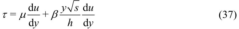
Numerically the shear stress is calculated as

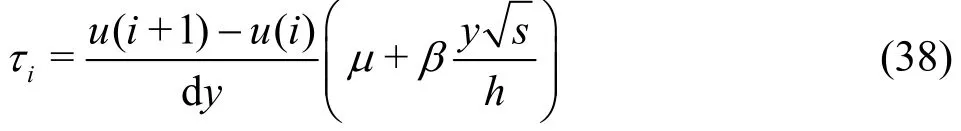
Fig. 8 Non-dimensional vertical shear stress distribution

Figure 8 represents the non-dimensional vertical shear stress distribution. The velocity in the lower vegetated layer in Tsujimoto and Kitamura[26]investigation is (0.2152 m/s) higher than in the present study(0.07 m/s). The maximum shear occurs at the interface as it happens in case of Tsujimoto and Kitamura[26].As the vegetation height and total depth of flow are different for the two situations, the non-dimensional interface differs numerically, but the shear stresses are maximum at the interfaces in both cases. This higher velocity in the lower vegetated zone results in higher bed shear stress which is evident from the Fig. 8. With the increase in the height from the bed, the turbulent stress increases which results in higher values of the shear in both the cases.

8. Conclusion

The streamwise velocity component through randomly distributed submerged rigid vegetation was experimentally measured using ADV at various locations within and outside the array. In the present study, the variation of the streamwise velocity component is plotted and compared with the results of submerged as well as emergent vegetation. The results are also validated with a proposed analytical model.The 1-D analytical model for flow through randomly distributed submerged rigid vegetation over an inclined plane bed is developed balancing the gravity force, drag force and the force due to the Reynolds stress acting on the fluid element. The turbulent stress model is employed to replace the nonlinear term of the stress with a linear relation between stress and the velocity gradient. The velocity field and shear stress are obtained solving the governing force balance equation numerically. The relevant dimensionless numbers have been identified and a correlation has been developed between these numbers which can be used to evaluate the value of the turbulent stress coefficient. The results obtained from the correlation are compared with the experimental results of the present study and with the previously reported investigations. The results indicate that the predicted velocity fields using the proposed model are in close agreement with the experimental results which demonstrates the validity of the correlation.