Min-hua Shu, Ke Chen, Yun-xiang You, Tian-qun Hu, Ren-feng Wang

State Key Laboratory of Ocean Engineering, Collaboration Innovation Center for Advanced Ship and Deep-Sea Exploitation Equipment, Shanghai JiaoTong University, Shanghai 200240, China

Abstract: The unsteady bearing forces of a propeller can be significantly affected by external transverse excitations. This paper numerically studies the unsteady variation characteristics of the bearing forces of a three-blade conventional propeller with external transverse excitations or without excitations. The dynamic mesh method combined with the RANS turbulence model is employed. The numerical simulation shows the frequency response in the frequency domain of KT, KQ under external transverse excitations. The frequency of the response is found always equal to twice of the excitation frequency. If the amplitude of the external transverse excitation keeps constant, the amplitude of the response increases with the increase of the excitation frequency. If the excitation frequency keeps constant, the amplitude of the response increases with the increase of the excitation amplitude, in a power-law relationship. The pressure distribution can be significantly affected by the external transverse excitation, leading to a high irregularity of the flow field.

Key words: External transverse excitation, unsteady bearing forces, excitation frequency, propeller, dynamic mesh method

Introduction

With the progress of the global ship technology,many new requirements for the vibration and noise performance have been proposed. As one of the three major sources of the ship noises, the propeller noise has an important impact on the total sound pressure level. The previous researches of the propeller noise mainly focus on the full-band of the total sound pressure level. But a large number of practical measurements on ships show that the high total sound pressure level is commonly caused by some particular components of medium or low frequencies. Because these particular noise components are closely related to the exciting force near the stern[1-2]and mainly produced by the propeller, systematic researches of the exciting force of the propeller are important for understanding the low frequency noise of the ships, as well as for the noise prediction and controls. Thus the exciting force of the propeller becomes an important issue in the naval architecture and the ocean engineering.

The unsteady bearing forces produced by the propeller in the non-uniform flow behind the ship stern are the direct excitation source of the ship vibration. The level and the variation of the unsteady bearing forces significantly affect the accuracy and the precision of the evaluation of the ship-radiated noise.Although model experiments[3-4]are effective ways to investigate the unsteady bearing forces, the scale effect due to the model size can be an unavoidable problem in addition to the remarkable discrepancies between the experimental results and the reality.Compared with the experiments, the numerical calculation methods have advantages in many respects,e.g. the propeller behavior may be simulated with real-scale models to provide details of the flow field.

The unsteady numerical simulation of the propeller was early proposed by Kerwin and Lee, by using the vortex lattice method. Then, the lifting surface method[5]and the panel method[6-7]based on the potential flow theory were developed to bring the simulations into a maturity stage. But the viscosity of the flow is ignored in the potential flow theory, with a certain deviation for a practical flow. In recent years,with the development of the viscous flow theory and the computation technology, the CFD based on the viscous numerical method becomes a major trend.Koushan and Krasilnikov[8], Zhang and Hong[9]analyzed the variation characteristics of the unsteady forces of the propeller in oblique flows. Hu et al.[10],Guo et al.[11], Lesfvendahl and Troeng[12]and Zhu et al.[13]adopted the viscous flow numerical method to investigate the hydrodynamics of the propeller in non-uniform and uniform flows. Zhang et al.[14], Li et al.[15]used the hybrid mesh technique to simulate the unsteady bearing forces of the propeller behind a ship with full appendages.

A recent focus is on the problems of the steady and unsteady hydrodynamics with external excitations,i.e. the vibration of the ship-shaft or the fluctuation effect of the flow field. Huang and Wu[16]studies the open water performance of a five-blade high-skewed propeller in the heave motion of the ship. Sharma et al.[17-18], Spyros et al.[19]analyzed the unsteady bearing forces of the propeller in the surge motion, the roll motion and the heave motion of the ship.

The influence of the external excitation on the propeller is very complex and is related with the non-uniform and unsteady flow field of the propeller,the fluctuation of the fluid and even the enhanced variation of the unsteady bearing forces of the propeller. So far, the variation characteristics of the unsteady bearing forces with different types of external excitations are still not very clear. This paper is devoted to the study of the variation characteristics of the unsteady bearing forces of the propeller with external transverse excitations. The RANS turbulence model and the dynamic mesh method are employed.

1. Numerical model

The governing equation, the model setup and the boundary conditions of the numerical method are introduced in this section.

1.1 Governing equations and turbulence model

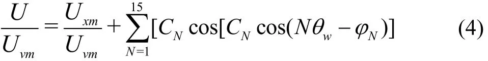
The dynamic mesh method is employed to simulate the flow field of the propeller. The mass and momentum conservations are expressed by the following governing equations[20-21]:

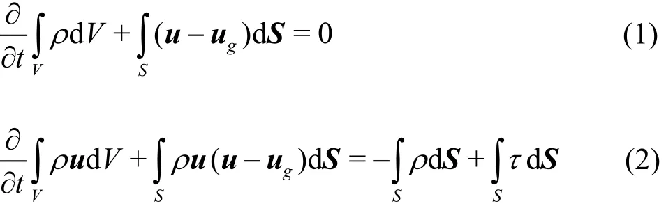
where μ is the dynamics viscosity coefficient.

The shear stress transport model SST k-ω is used as the turbulence model, as employed in previous studies[22-23].

1.2 Physical model

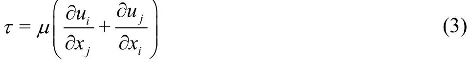
A three-blade conventional propeller DTMB 4119 is selected as the physical model. Its basic parameters are shown in Table 1. A schematic diagram of the numerical model is shown in Fig. 1. A moving local coordinate system o-xyz is defined on the propeller and will have the same rotation and vibration as the propeller during the simulation. The origin of the coordinate o is the geometric center of the propeller which is also the intersection point of the propeller disk plane and the shaft axis. The x-axis coincides with the shaft axis, pointing to the downstream direction. The vertical z-axis is in the upward direction and y-axis lies in the horizontal plane. The whole computation domain is a cylinder and is mainly divided into two parts, i.e., the inner cylinder containing the propeller and the outer zone. A stationary global coordinate system O-XYZ is used to monitor the motion of the point o. The parameters of the domain are shown in Fig. 1. The surfaces of the blades and the hub are discretized by triangular elements and are wrapped by multilayer prismatic boundary layer grids. To obtain more precise results,the mesh is refined on the leading edge, the trailing edge and the blade tip. The inner cylinder zone is filled with tetrahedral elements while the outer zone is filled with hexahedron elements.

Table 1 Parameters of the DTMB 4119 propeller

1.3 Boundary conditions

Jessup[24]conducted an experimental study of the unsteady bearing forces. The computation results are compared with those of the experiments, with the parameters the same as those of the Jessup’s. According to the experimental conditions[24], we have the advance coefficient J =0.833, the rotational speed n =10 r/s, i.e., the shaft frequency is 10 Hz, and the 9-cycle non-uniform incoming flow produced by a 9-cycle wire mesh screens. The expression of the incoming flow is given by

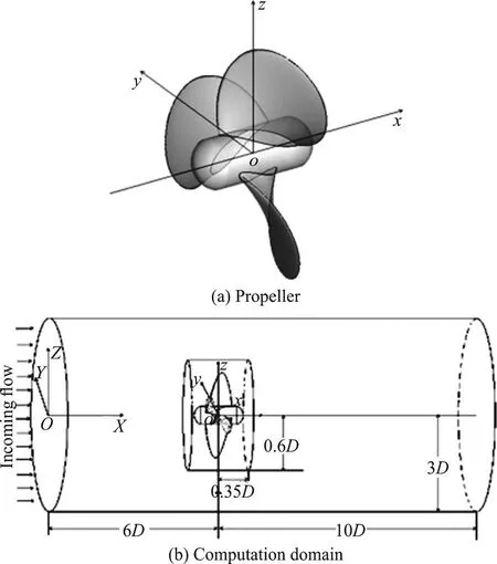
Fig. 1 Schematic diagram of the model and the computation domain

where Uvmis the volume mean velocity, CNthe coefficient,wθ the angle of the upstream with the propeller axis, positive in the clockwise direction, N the harmonic number in the axial wake inflow,Nφ the phase angle of the Nth harmonic of the axial wake inflow and Uxmthe circumferential average axial velocity, which is the mean value of the axial velocities on a circumference with a certain radial position. The parameters of Eq. (4) can be found in Ref. [24].

Figure 2 shows the circumferential distribution of the non-uniform incoming flow at different radial positions calculated by Eq. (4). At 0.3R (Ris the tip radius of the propeller), the fluctuation of the velocity distribution is relatively small and the maximum drop between the peaks and the valleys is 0.05. With the increase of the radial distance, the 9-cycle feature becomes more and more distinct. The maximum drop between the peaks and the valleys is 0.20 at 0.5R,0.32 at 0.7Rand reaches 0.43 at 0.9R, showing the growth trend. The 9-cycle non-uniform incoming flow is loaded at the left surface of the cylindrical computation domain as the velocity inlet boundary. The right surface of the domain is under the pressure outlet boundary condition. The sides of the cylindrical domain are assumed to be the velocity inlet with the volume mean velocity Uvm. The blades and the hub are defined as a wall.

Fig. 2 The circumferential distributions of non-uniform incoming flow at different radial positions

1.4 Motions of the model

In this work, the propeller has two motions, i.e.,the pivot movement driven by the shaft and the vibration along the Y-axis caused by the external transverse excitation.

For the pivot of the propeller, under the condition of the non-uniform incoming flow and with the parameters of the propeller, the rotational speed n is given by

where J is the advance coefficient and D=2R is the diameter of the propeller.

For the vibration along Y-axis, the displacement is expressed as

where A = Ymax/D is the dimensionless amplitude,Ymaxthe maximum displacement, fethe excitation frequency and t the time. The velocity of the vibration is given by

Equations (5), (7) are applied to the wall boundary of the propeller, to move the propeller.

It should be noted that the incoming flow is not influenced by the excitation and the reduced frequency of the problem is K = Ninθb=3.375, where Ninis the harmonic number of the non-uniform incoming flow and θbis the blade semi-chord projected angle[24].

2. Analysis of unsteady bearing forces

Two unsteady forces, namely the thrust and the torque, are investigated in this work, represented by the thrust coefficient KT, the torque coefficient KQ.The definitions of these two coefficients are as follows:

where Txis the axial thrust, Qxis the axial torque.

2.1 Verification of the numerical method

For the computational study, the quality of the grid is extremely important for the results. The grid independence is first analyzed for the case without excitation. Here three sets of grid of different qualities are considered. The numbers of the elements in the three cases are shown in Table 2.

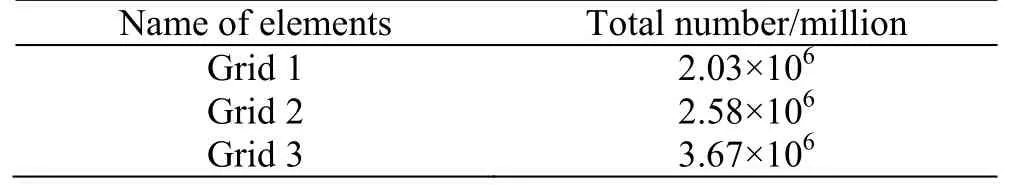
Table 2 The total numbers of three sets of grid

Figure 3 shows the time-series of the unsteady bearing forces of the propeller, namely KT, KQ,associated with the three sets of grid. It is shown that the results of KTassociated with the three sets of grid generally agree with each other and the results of KQare also similar. Moreover, the results of Grid 2,Grid 3 have better agreements in details, especially, at the peaks and the valleys of the curves.

As previously mentioned, Jessup[24]conducted an experimental study of KT, KQwithout the external excitation. In the experiments, KT, KQboth have three peaks in the frequency domain, corresponding to the harmonic number N1=3, 6 and 9. In our results,these three peaks are also found and we further compare the numerical results with the experimental data. Table 3 lists the relative errors between the experiments and the computations for the three sets of grid for the harmonic number N1=0 (average value),3, 6 and 9.

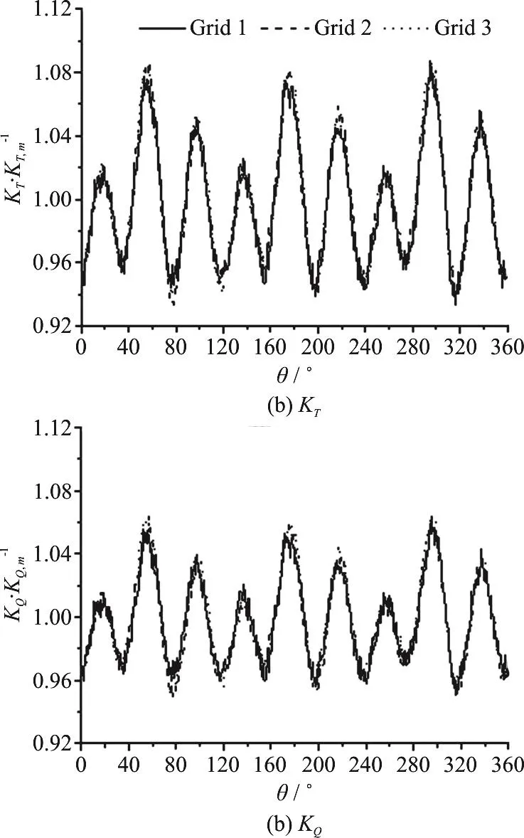
Fig. 3 Time-domain characteristics of the unsteady bearing forces of a propeller in three sets of grid

For the harmonic number N1=0, 6 and 9, the errors are smaller than 10%. But for the harmonic number N1=3, the errors are over 20%. Such discrepancies can also be found in Hu’s numerical study[16]obtained with the sliding mesh method. One explanation may be that the lower-order harmonic components of the non-uniform incoming flow wake are more easily to dissipate when the fluid moves from the inlet to the propeller disk plane, which can not be precisely simulated in computation. Another plausible reason is that, with the facility in the experiments (the width of the tunnel of 0.67 m is only about twice of the propeller disk diameter of 0.30 m),the flow reflection from the tunnel wall would inevitably enhance the low frequency components of the flow, leading to a larger response for the low-order harmonic number N1=3, while the reflection is ignored in the simulation.

As no experimental study is reported yet in this respect, the computational method for the vibrationswill be verified by comparing the results obtained with the three sets of grid under an external transverse excitation. The results of KT, KQare listed in Table 4 for the case of an excitation with frequency fe=10 Hz and amplitude A =1.311× 10-2. With the external transverse excitation, a new response frequency appears. From the comparison, the results of Grid 2, Grid 3 are very close to each other but noticeably different from those of Grid 1. Therefore,Grid 2 is chosen for subsequent studies in view of a balance of the efficiency and the precision of the calculation.

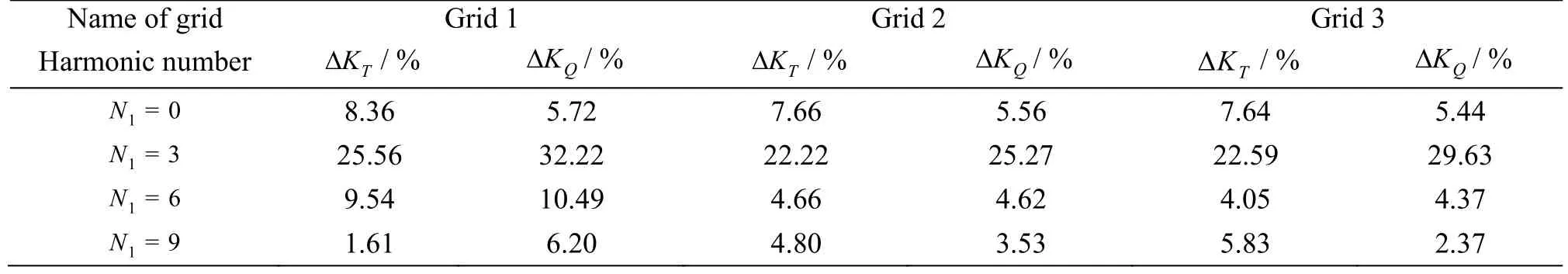
Table 3 Relative errors of every order harmonic of the unsteady bearing forces obtained with three sets of grid

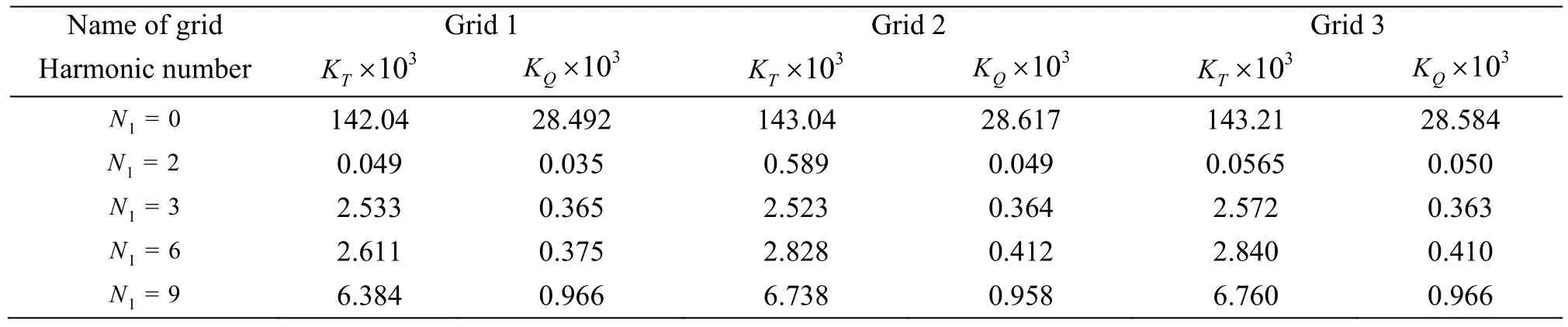
Table 4 The results of KT, KQ obtained with three sets of grid when =10 Hz ef , 2=1.311 10A × -

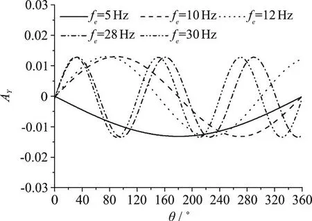
Fig. 4 Time-series for the Y - axis position of the geometric center of the propeller under transverse excitations with different frequencies when A = 1.311×10 2

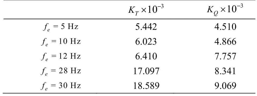
Table 5 Average differences between each excitation and the case of no excitation

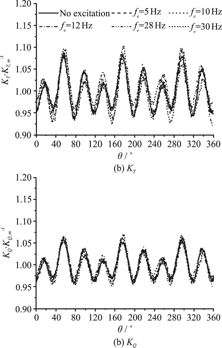
Fig. 5 Time-series for KT, KQ for no excitation and 5 transverse excitations with different frequencies, when A=1.311× 10-2

2.2 Influf excitatio n frequency

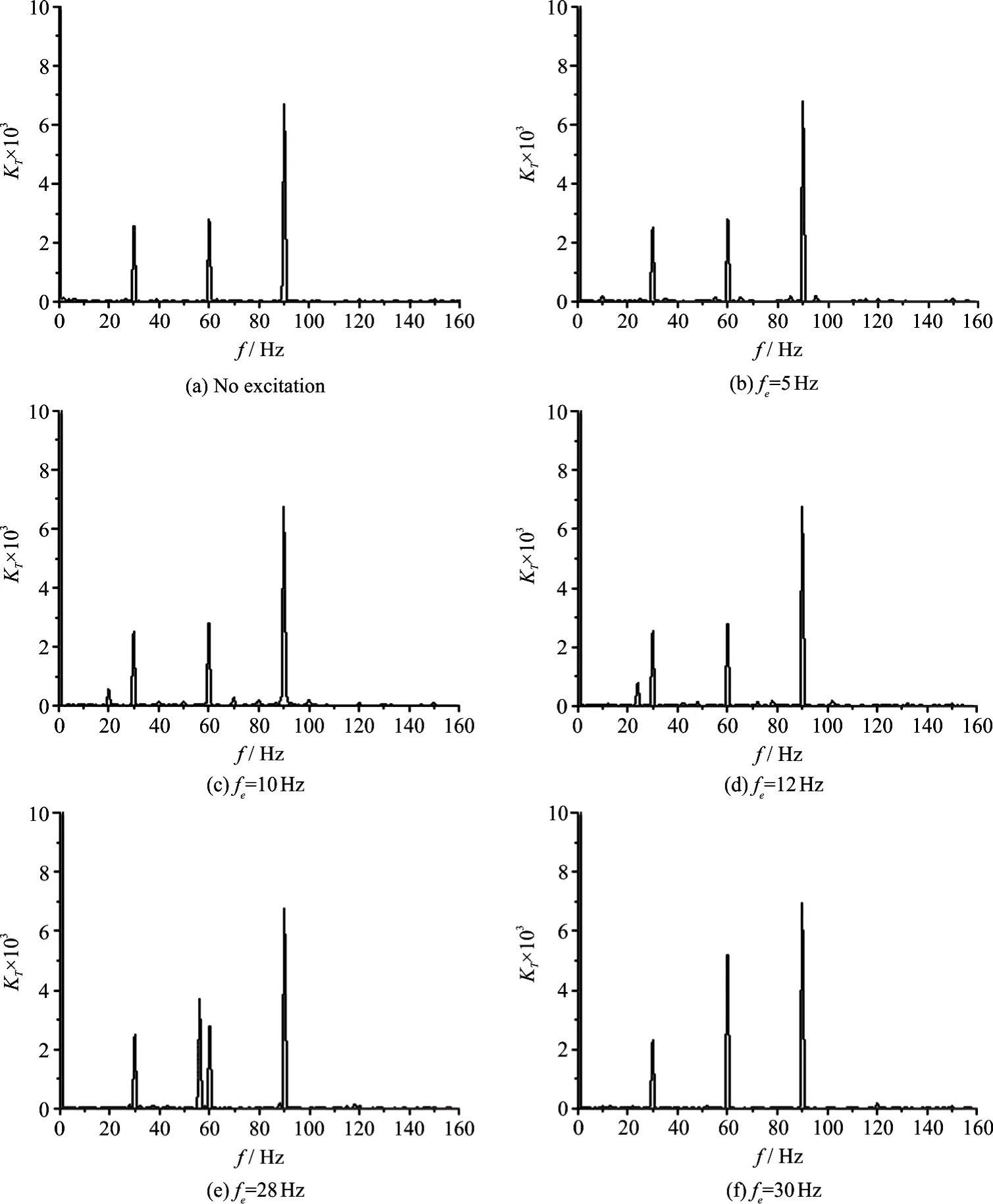
Fig. 6 Frequency-domain characteristics of KT for no excitation and five transverse excitations with different frequencies when A=1.311× 10-2

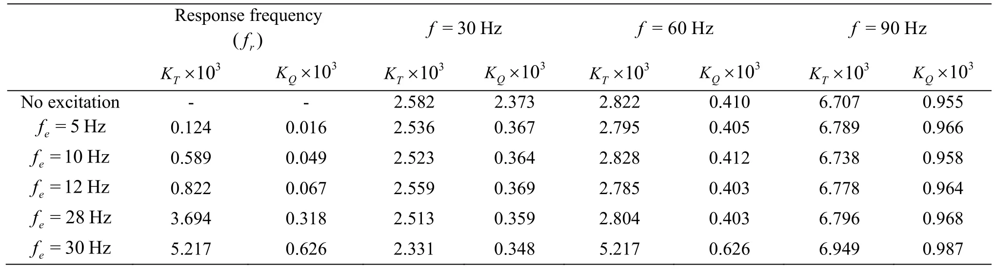
Table 6 The results of KT, KQ for no excitation and five transverse excitations with different frequencies

Tostudythevariationch aracteristicsofthe unsteady bearing forces KT, KQfor external transverse excitations with different frequencies, five excitation frequencies feare considered, i.e., fe=5 Hz,10 Hz, 12 Hz, 28 Hz and 30 Hz when the excitation amplitude A =1.311× 10-2keeps unchanged. Figure 4 presents the Y-axis position of the point o, i.e.,the geometric center of the propeller for the five external excitation frequencies in one cycle of the propeller rotation and the corresponding duration is Δ t=0.1s . In one cycle of the propeller rotation with the excitation frequency fe=5Hz, the geometric center leaves the equilibrium position AY=0,moving to the direction of -AYand then goes back to the position AY=0 after reaching the maximum displacement, i.e., the geometric center goes over a half cycle of the vibration along the Y-axis. With the excitatio n freq uenc y fe=10 Hz, th e g eome tric center positiongoesoveranentirecycleofthevibration along the Y-axis during a rotation cycle. Actually,the vibration frequencies of the geometric center of the propeller are exactly the same as the excitation frequencies and the dimensionless vibration amplitude is equal to the excitation amplitude. The results suggest that the Y-axis vibration of the propeller is successfully realized in the numerical simulation for the external transverse excitations with different excitation frequencies.

Figure 5 shows the time-series for KT, KQfor no excitation and for five external transverse excitations with different frequencies when A=1.311×10-2. For both, K, the variation trends of theQsix curves representing different cases are similar. In Fig. 5, each curve has nine peaks, which obviously embodies the characteristics of the 9-order angular frequencies, related to the 9-cycle non-uniform incoming flow. According to their values, the nine peaks can approximately be classified into three classes and each is uniformly located in the 360°-zone,with a 120°-cycle, i.e., N1=360°/120°=3, as related to the blade pass frequency (BPF). Moreover,Fig. 5 shows that the curves for various excitations do not precisely coincide with the curve for no excitation and the deviations are varied. To quantitatively describe the deviations, the average differences between the curves for various excitations and for no excitation are calculated. Table 5 shows the results of the average differences, indicating that the deviation increases with the increasing excitation frequency.

The characteristics of KT, KQin the frequency domain are also important. Here the FFT spectrum analysis method is adopted to reveal the frequency domain characteristics of the unsteady bearing forces. Figure 6 shows the frequency characteristics of the thrust coefficient KTunder different excitation conditions, i.e. with no excitation,and with the excitation frequency fe=5 Hz, 10 Hz,12 Hz, 28 Hz and 30 Hz when A=1.311× 10-2.

According to the previous study[25], the frequency responses in the unsteady thrust and torque are obtained from those wake harmonics which are multiples of the number of blades (kZ1). Therefore,when there is no external excitation, three significant frequency components are observed in the frequency domain with the frequency f=30 Hz, 60 Hz and 90 Hz.The component for f =90Hz is dominant due to the coupling between the dominant 9th harmonic of the incoming flow and the 3rd harmonic of the BPF. The components for f =30Hz , f =60 Hz are partially due to some 3rd and 6th harmonic contents in the incoming flow and are the 1st and 2nd harmonics of the BPF.

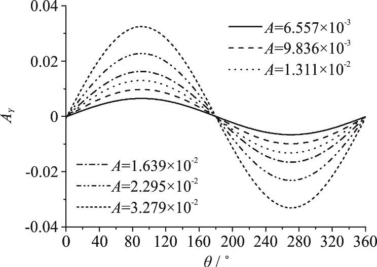
Fig. 7 Time-series for the Y-axis position of the geometric center of the propeller for six transverse excitations with different amplitudes when fe=10 Hz

With an external transverse excitation, the components of the frequencies f=30 Hz, 60 Hz and 90 Hz still exist while an extra frequency component appears. According to the observation, the extra response frequency fris independent of the harmonics of the BPF and the incoming flow, but exactly the twice of the excitation frequency (i.e., fr=2fe).It is because that the transverse movement of the propeller is symmetric along Y-axial. Table 6 shows the frequency responses associated with different excitation conditions. It is shown that the external transverse excitations barely affect the characteristics of the frequency components for f=30 Hz, 60 Hz and 90 Hz, but it will affect the characteristics of the frequency fr. And the amplitude corresponding to frbecomes larger with the increase of the excitation frequency. When the excitation frequency fe=30 Hz, it coincides with the 2nd harmonic of the BPF.Thus in this case, the amplitude at f =60 Hz is the superposition of the BPF and the frequency response,becoming remarkably higher than those in other cases.

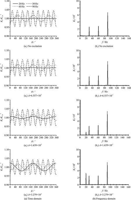
Fig. 8 Time-series and frequency-domain characteristics of KT for no excitation or three transverse excitations with different amplitudes when fe =10 Hz

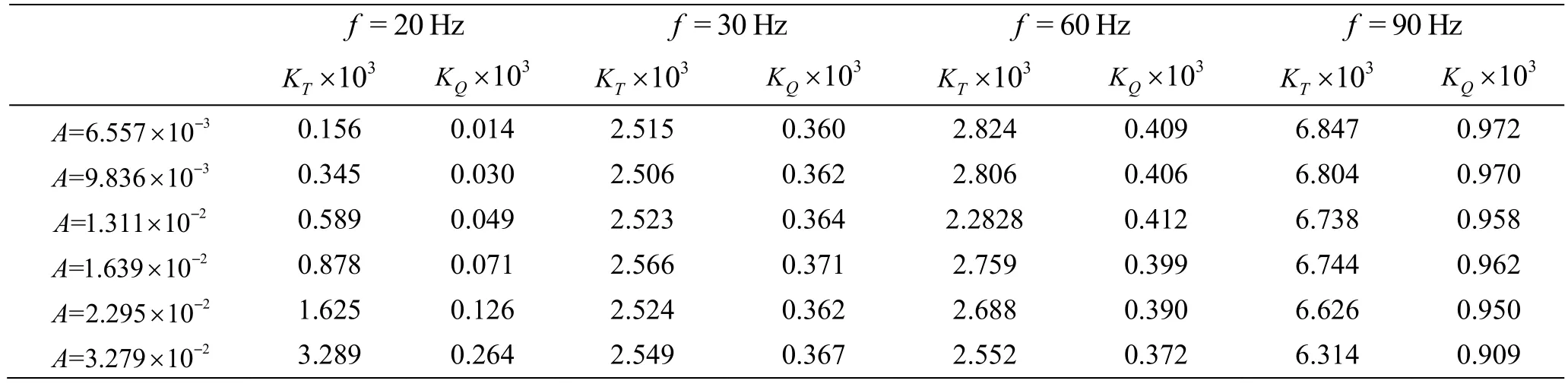
Table 7 The results of KT, KQ for different excitation amplitudes

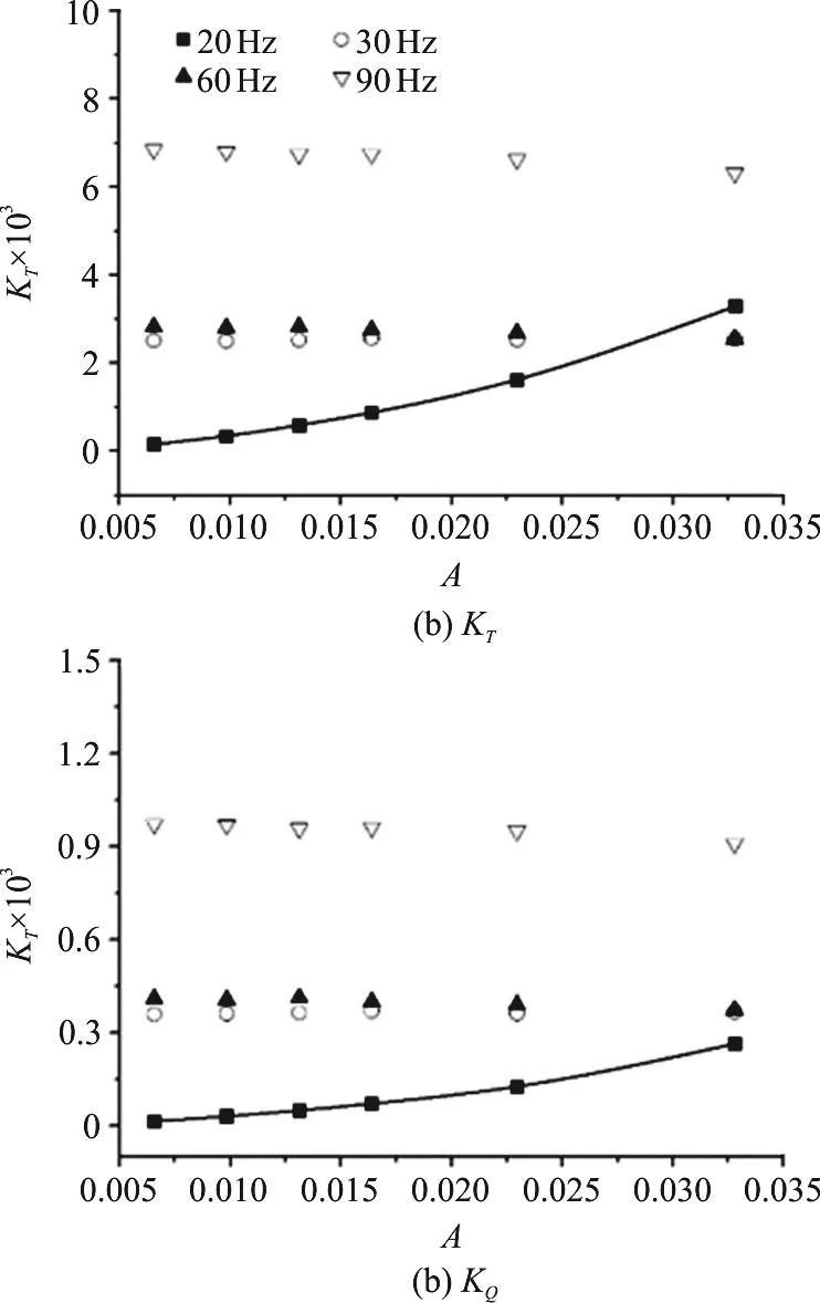
Fig. 9 Scatter diagram for each frequency component of KT,K Q against the excitation amplitudes

Moreover, the superposition of the BPF and the frequency response of the excitation cannot be linear.The average value of the amplitude at f =30Hz is 2.542 in other cases and the amplitude of the frequency response of the excitation is 3.69 when fe=28Hz . In view of the growth trend of the amplitude of the frequency r esponse pr eviously observed, the linearsuperpositionisexpectedtoform an amplitude larger than 6.232 whereas it is only 5.22,implying a non-linear superposition between the BPF and the excitation. The characteristics of KQare very similar to those of KTand are not necessary to be repeated here.

2.3 Influence of excitation amplitude

To study the influence of the excitation amplitude on the unsteady bearing forces, six excitation amplitudes are considered in this section, namely A=6.557× 10-3, A =9.836× 10-3, A=1.311× 10-2,A=1.639× 10-2, A =2.295× 10-2and A=3.279×10-2with the excitation frequency fe=10 Hz . Figure 7 shows the Y-axis position of the geometric center of the propeller for the six external excitation amplitudes in one cycle of the propeller rotation and the corresponding duration is Δt =0.1s . As the excitation frequency is equal to the shaft frequency 10 Hz,the propeller is expected to experience one cycle of the vibration along the Y-axis during one cycle of the rotation in each case, as is affirmed by Fig. 7.According to the observation, the dimensionless vibration amplitude of the geometric center of the propeller is consistent to the excitation amplitude,indicating that the vibration of the propeller is realized in the numerical simulation for the external excitations with difference amplitudes.

According to the analysis in the frequency domain, the original time-series of KT, KQare mainly composed of the components for f= 30 Hz, 60 Hz,90 Hz, i.e., for the first three harmonic frequencies of the BPF, and for the twice of the excitation frequency 2 fe= 20 Hz . Thus, the original time-series can be decomposed by means of the band-pass method.Figure 8 shows the decomposed time-series curves and the frequency domain characteristics of KT. In the case of no excitation on the propeller, the component for 20 Hz associated with the external transverse excitation does not appear in Figs. 8(a1),8(b1), and only the components for 30 Hz, 60 Hz and 90 Hz, corresponding to the first three harmonic numbers of the BPF, can be seen. With the external transverse excitation, the 20 Hz component appears and its amplitude will be affected by the variation of the excitation amplitude. The characteristics of KQare similar.

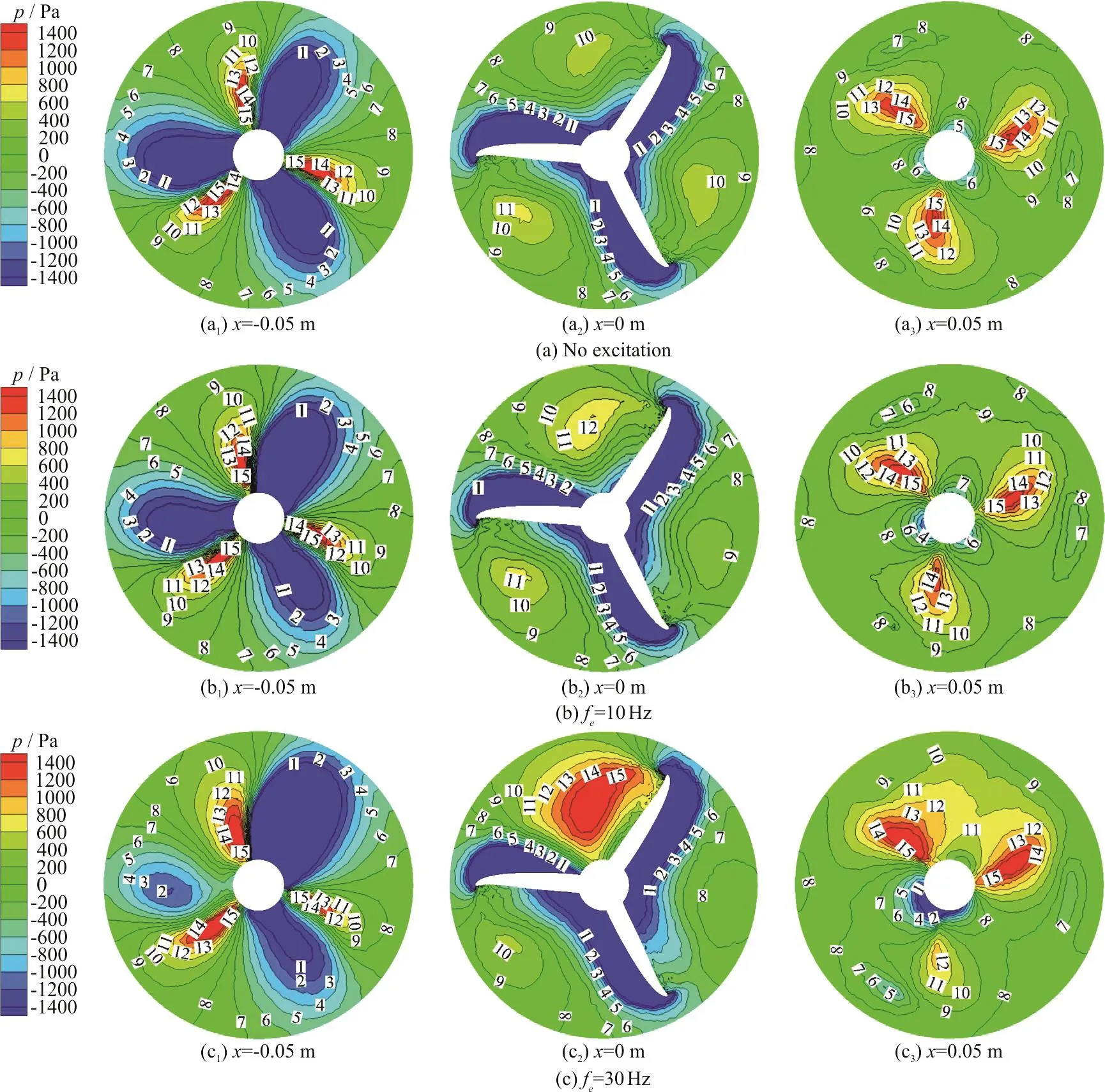
Fig. 10 (Color online) The pressure distributions on three disks of the flow field of propeller with no excitation and with two transverse excitations of different frequencies when A =1.311× 10-2

Table 7 shows the data of the amplitudes associated with different frequency components for different excitation amplitudes for KT, KQ. Figure 9 shows the scatter diagram of the data in Table 7.According to Table 7, Fig. 9, the amplitudes for the components of 30 Hz, 60 Hz and 90 Hz almost keeps unchanged when the excitation amplitude changes and the amplitude for the 20 Hz component shows a growth trend with the increasing excitation amplitude.

Using the regression analysis and ignoring the data without excitation, the variations of KT, KQagainst the excitation amplitude are obtained as follows:

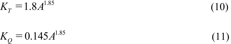
Therefore, KT, KQboth have a power-law relationship with the excitation amplitude, with the same power 1.85 but different coefficients.

3. Analysis of pressure distribution

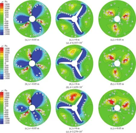
Fig. 11 (Color online) The pressure distributions on three disks of the flow field of propeller with no excitation and with three transverse excitations of different amplitudes when fe =10 Hz

With the external transverse excitations, the irregularity of the pressure distribution around the propeller will be greatly enhanced, leading probably to the growth of the noise level in the flow field. In this section, the pressure distributions for different excitations are analyzed. Figure 10 illustrates the pressure distributions on the cross-sections of the inner zone of the computation domain at x = - 0.05 m,x =0 m and x =0.05m for the excitation frequency fe=5 Hz, 30Hz and for no excitation with the excitation amplitude A=1.311× 10-2. In the case without excitation, the entire cross-section can be divided into three equal sectors with a 120° central angle and the pressure distribution in each sector is almost the same despite of the x-axis position,showing a relatively good regularity. In the case of the 10Hz excitation frequency, the slight variation of the pressure distribution appears at the disk plane of the propeller (x=0 m) while the variation can be hardly observedattheotherplanes(x = - 0.05 m, x=0.05 m). When the excitation frequency reaches 30 Hz,the variation of the pressure distribution becomes significant on each cross-section, indicating a strong irregularity of the flow field.

Figure 11 shows the pressure distributions on the cross-sections at x = - 0.05 m , x=0 m and x=0.05 m for the excitation amplitude A=6.557×10-3,1.639×10-2and 3.279×10-2when the excitation frequency fe=10 Hz . For the amplitude A=6.557×10-3, the pressure distribution is very similar to that without excitation, as shown in Fig. 10 and the change of the pressure can hardly be observed. Then the slight variation of the pressure field begins to be observed on the plane at x=0 m when the excitation amplitude reaches A=1.311× 10-2(Fig. 10) while the pressure on the planes at x = - 0.05 m and x=0.05 m seems not to be influenced. When the amplitude becomes A=3.279× 10-2, the variation of the pressure can be clearly seen in the figure on each plane,which means that the flow field is highly irregular due to the vibration of the propeller.

Therefore, the pressure distribution of the flow field can be significantly affected by the propeller vibration due to the external transverse excitation. The irregularity of the flow field grows more and more noticeable while the excitation frequency or the amplitude increases, according to the observation.

4. Conclusions

Based on the dynamic mesh method and the RANS turbulence model, the effects of the external transverse excitation on the unsteady bearing forces of a three-blade conventional propeller are numerically investigated in this paper. The grid independence and the numerical method are verified by comparing the computational results of three grid sets and the results in previous studies.

It is shown that three significant frequency components are found in the frequency domain of KT,KQvariations, i.e., fe=30 Hz, 60 Hz and 90 Hz,which are, respectively, consistent to the blade pass frequency (BPF), the 2nd and 3rd harmonics of the BPF. With an external transverse excitation, a frequency response with a frequency twice of the excitation frequency is observed and, in most cases,the amplitude of the frequency response will increase with the increase of the excitation frequency if the excitation amplitude keeps unchanged. In some special cases, the frequency of the response may coin cide with fe=30 Hz, 6 0 Hz or 90 H z and the twofrequencycomponentswillhaveanonlinear superposition. If the excitation frequency keeps unchanged, the amplitude of the frequency response will increase with the increase of the excitation amplitude with functional relationships, i.e., KT=

Moreover, the pressure distribution of the flow field can be affected by the propeller vibration due to the external transverse excitation. The irregularity of the flow field grows while the excitation frequency or amplitude increases, which may lead to a higher level of the noise in the flow field.

Therefore, the characteristics of the external transverse excitation should be considered in the design of a propeller in order to avoid the enhancement of the variation characteristics of the unsteady bearing force and the irregularity of the nearby flow field.